1. Introduction
Automated building roof contour extraction in particular has been studied for over three decades. Extraction methods can be based on either LiDAR data, photogrammetric information, or a combination of these data types.
Methods based on photogrammetric data have been proposed for over 20 years. For example, Fua and Hanson (1987) have proposed a process for locating and outlining complex rectilinear cultural objects (buildings) in aerial images. More recently, Müller and Zaum (2005) have proposed a technique for detecting buildings in aerial images using a region-growing segmentation algorithm combined with a classification procedure for distinguishing between buildings and vegetation.
In addition, Akçay and Aksoy (2008) presented a novel method for automatic detection of building and other objects (roads and vegetation) in high-resolution images by combining spectral information with structural information exploited by using image segmentation. Very recently, Ferraioli (2010) proposed a stochastic approach for building edge detection in multichannel InSAR imagery. Building edges are detected by modeling the image as a Gaussian Markov Random Field with local hyperparameters.
S?rmaçek and Ünsalan (2011) also presented a probabilistic approach but for detecting buildings in aerial and satellite images. Local feature vectors are extracted and used as observations of the probability density function to be estimated, from which building locations are detected in the image.
Jwa et al. (2008) focused on the regularization of noisy building roof contours by dynamically rearranging quantized line slopes in a local shape configuration and globally selecting optimal outlines based on minimum description length principles. A Bayesian approach for automatically constructing building footprints from a pre-classified LIDAR point cloud is presented by Wang et al. (2006). The proposed method determines the most probable building footprint by maximizing the posterior probability using linear optimization and SA (Simulated Annealing) techniques.
Since its introduction, simulated annealing has received significant attention in the last two decades and has been applied to optimization problems in diverse areas (Collins et al., 1988; Glover, Greenberg, 1989; Rutenbar, 1989; Eglese, 1990; Shutler, 2003). Kirkpatrick et al. (1983), Cerny (1985) and McCormick, Powell (2004) showed that a model for simulating the annealing of solids, proposed by Metropolis et al. (1953), could be used for optimization of problems, where the objective function to be minimized corresponds to the energy of states of the metal.
In this paper, a method by SA for building roof contours identification from LiDAR-derived DSM (digital surface model) is proposed. Our method is based on the concept of first extracting aboveground objects and then identifying those objects that are building roof contours. The method uses two steps. In the first step, we used standard image processing algorithms to segment the DSM into aboveground and background regions, followed by the application of a contour following algorithm and the Douglas-Peucker algorithm to generate polyline representations for the aboveground regions.
Second, building roof contours are identified from among the aboveground objects by optimizing a Markov-random-field-based energy function that embodies roof contour attributes and spatial constraints. The optimal configuration of building roof contours is found by minimizing the energy function using a simulated annealing algorithm.
2. Simulated Annealing Algorithm for identification of building roof contours
To minimize the energy function U, several optimization algorithms can be used to properly obtain the optimal solution (p1, …, pn). We used the SA algorithm because it is usually effective in finding the global minimum, even when the energy function has local minima (Kopparapu and Desai, 2001).
2.1 Lidar Data preprocessing
The proposed method for automatic extraction of aboveground regions uses the following steps: DSM generation from a LiDAR point cloud by interpolating the LiDAR point cloud into a regular grid. We used the nearest-neighbor interpolation method, mainly because it allows the original heights to be maintained within the DSM.
DSM segmentation into aboveground and ground objects, segmentation is accomplished in two steps: segmentation of the DSM using the recursive splitting technique (Jain et al., 1995) and refinement of the segmentation by a region merging. The next step consists of grouping adjacent regions of similar heights in such a way that over-segmentation that is typical of the recursive splitting technique is minimized and the resulting regions correspond to either ground or aboveground objects.
Considering that we are interested in objects that are at least 3m tall (i.e., buildings), our algorithm initially searches for two segments for which the difference between their mean heights is greater than a threshold value (e.g., 2.5m). The fundamental result of the segmentation process is a binary grid where ground grid points are assigned a zero value and aboveground grid points are assigned a value of one.
Because our strategy for identifying building roof contours requires that aboveground regions (buildings and other objects - e.g. trees) be represented by polylines, we applied sequentially a contour following algorithm that is, in essence, the same procedure described by Ballard and Brown (1982) for generating ordered lists of contour points.
Finally, we applied the Douglas-Peucker algorithm to generate polyline representations for the ordered lists of contour points obtained using the contour following algorithm.
2.2 Formulation of energy function
In an MRF (Markov Random Field) model, the sites S={1, …, n} are related to one another through a neighborhood system defined as , where is the set of sites neighboring i. According to the Hammersley-Clifford theorem, an MRF can be characterized by a Gibbs probability distribution (Kopparapu and Desai, 2001), i.e.:
P(x) = 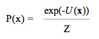 (1)
(1)
Z =  (2)
(2)
where, x is a configuration of a random field X, is the set of all possible configurations of the random field X, and U(x) is an energy function, which can be expressed as:
 (3)
(3)
Equation 3 shows that the energy function is a sum of clique potentials (Vc(x)) over all possible cliques c C. A clique c is a subset of sites in S in which every pair of distinct sites are neighbors. The value of Vc(x) depends on the local configuration of clique c.
Polylines representing building roof contours can be found by analyzing the aboveground region polylines. We formulated this problem as an MRF where the energy function takes the following mathematical form:
(4)
In Equation 4, is a parameter that varies over [0; 1] and converges to one if the region is interpreted as a building roof contour; otherwise, pi converges to zero. In addition, n is the number of regions, and are positive constants that express the relative importance of the following energy terms:
Rectangularity energy. This term favors rectilinear regions (polylines) defined as straight lines that are parallel or perpendicular to one another. This geometry is modeled by the rectangularity attribute, which is defined as:
![]() (5)
(5)
where is the angle between the two main directions of the region .
We used the following algorithm to compute the two main directions of a region polyline :
1) subdivide the trigonometric circle into 24 sectors ranging over [0º; 15º[, …, [345º; 360º];
2) create a 24-cell array and initialize it to zero;
3) select a straight-line segment of the region polyline and compute its direction d and the length l;
4) extract the integer part (n) of length l;
5) identify the sector containing the direction d and increment the corresponding cell n times;
6) repeat steps 3 to 5 for all remaining straight-line segments of the region polyline .
The two main directions of the region polyline are the average angles of the two sectors corresponding to the two most abundant cells. The most abundant cell corresponds to the primary direction (for example, it is 7.5º if the first sector is the most abundant one).
The optimal value of attribute is one, meaning that the region polyline contains only pairs of straight lines that are either parallel or perpendicular to one another. Because we searched for the minimum of the energy function U, the solution ( is 90º for a perfectly rectilinear representation of a building) forces to converge to one if we consider only the rectangularity criterion.
Area energy. This term favors larger regions, and therefore, a larger region corresponds to a smaller area energy term. The parameter starts with a random value over [0;1] and it is expected to converge slowly to one for a region representing a building. During the convergence of , the larger the area ( ) of region , the lesser the area energy term. The importance of the area decreases when . When = 0, the area does not contribute anymore, but will not change anymore. To avoid grouping small regions, the area energy term is set to a large positive value if the area is below a given threshold (e.g., 30m2).
Spatial energy. The third energy term benefits polyline regions that have primary directions that are approximately parallel or perpendicular to one another. In this term, is the angle between the main directions of polyline regions and . Moreover, because the spatial energy term is also a second-order clique energy term, it is necessary to define the neighborhood system as:
![]() (6)
(6)
in which the function dist is given by the Euclidean distance between the centroids of the two regions and and d is a distance threshold below which the region is considered to be in the neighborhood of the region . The formulation of the spatial energy term was inspired by formal settlements showing regular grids. The optimal contribution from this energy term would arise for a region configuration having building roof contours that are closely parallel or perpendicular to one another. In this case, ![]() ~ 0º or
~ 0º or ![]() ~ 90º, and pi and pj are forced to converge to one.
~ 90º, and pi and pj are forced to converge to one.
Entropy energy. This is the entropy of (which can be interpreted as the probability of region Ri being a building roof contour). The purpose of this term is to force to converge to either one or zero.
2.3 Energy function minimization
To minimize the energy function U, several optimization algorithms can be used to properly obtain the optimal solution (p1, …, pn). We used the SA algorithm because it is usually effective in finding the global minimum, even when the energy function has local minima (Kopparapu and Desai, 2001).
A basic SA scheme (Starck, 1996) was used, which can be summarized in three main steps:
1) Initialize the initial temperature (T0) and the initial solution (p0). The vector p0 can be randomly generated from a normal distribution and U0 is computed from p0 by using Equation 4;
2) Randomize and analyze, taking into consideration is the current solution and ti is the current temperature. If , ![]() then accept the new configuration pj; otherwise, accept pj only with the probability
then accept the new configuration pj; otherwise, accept pj only with the probability ![]() . Repeat until the thermal equilibrium is reached, i.e.
. Repeat until the thermal equilibrium is reached, i.e. ![]()
3) Compute the new temperature ![]() , where
, where ![]() . If the system is frozen (
. If the system is frozen (![]() ), where Tuser is supplied by an operator, stop; otherwise, go to step 2.
), where Tuser is supplied by an operator, stop; otherwise, go to step 2.
At the end of process, the global minimum is and the corresponding optimum solution is p = pj. The best configuration of building roof contours corresponds to the region Ri having parameter P i equal to one.
3. Experimental Results
Here, we present and analyze the results obtained using the proposed method. The input data for our method are composed of a set of irregularly distributed laser scanner points each having a UTM (Universe Transverse Mercator) coordinate (E, N) and an orthometric height (h). Each point also has a laser pulse return intensity (I), which is useful for visualization purposes. The LiDAR density is about 2 points per m2. The data set used here was obtained from Curitiba, Brazil.
To experimentally verify the performance of the proposed method, 2 different test areas were selected. The nearest-neighbor interpolation method was used for generating a 70-cm-resolution DSM for each test area. We used the SPRING freeware developed by INPE (National Institute for Space Research), Brazil, which is available at http://www.dpi.inpe.br/spring/english/index.html.
The remaining processing steps were developed in Builder C++ 4.0. Constants of the energy function U were empirically determined by trial and error, resulting in the following values: ![]() and
and ![]() Other parameters were determined similarly and the obtained values are:
Other parameters were determined similarly and the obtained values are: ![]() These values were kept constant in all of our experiments.
These values were kept constant in all of our experiments.
To assess the quality of the obtained results, the extracted building roof contours were numerically compared to reference contours that were manually digitalized based on an intensity image. This image was generated by interpolating the laser pulse return intensities into a regular grid. The numerical assessment of the quality of the results was based on the following parameters (Ruther et al., 2002):
![]() (7)
(7)
![]() (8)
(8)
where BER is the building extraction rate parameter; CB is the number of contours correctly identified as buildings; FP is the number of false positives; ACi is the area completeness parameter for the ith building roof contour; Ai is the area of the ith extracted building roof contour; and Bi is the area of the ith reference building roof contour.
Below, we present and analyze the results obtained for the 2 test areas. Figure 1(a) shows a 3D visualization of the test area 1 DSM. Five buildings can be readily identified, with three of them being aligned and almost attached. Figure 1(a) shows another building, which is not identifiable in Figure 1, near the upper-right corner of the intensity image.
Figure 1 - Results for test area 1. (a) Three-dimensional visualization of the test area 1 DSM; (b) Aboveground regions; (c) Contours of the aboveground regions; and (d) Identified building roof contours.
The detected aboveground regions present in test area 1 are displayed in Figure 1(b) using a binary grid (dark areas). The corresponding polylines are visualized in Figure 1(c). Figures 1(b) and 1(c) also show that an aboveground region representing the building surrounded by trees near the upper-right corner of the intensity image (see the arrow in Figure 1(a)) was not detected. Also note this corresponding area in Figure 1. Figure 1(d) shows that the proposed method correctly identified all of the buildings, with the exception of the building that was not detected in the first step of our method. Please note that all extracted buildings had relatively regular shapes and favorable spatial orientation (approximately parallel or perpendicular to one another). These are key characteristics to correctly identifying buildings by minimizing the proposed energy function. Please also note that the three aligned buildings were merged in the first step of our method (see Figures 1(b) and 1(c)). As a result, only a single long building is identified in the second step.
Figure 2 (a) shows a 3D visualization of the test area 2 DSM, the test area shows a more complex configuration when compared to the test area.
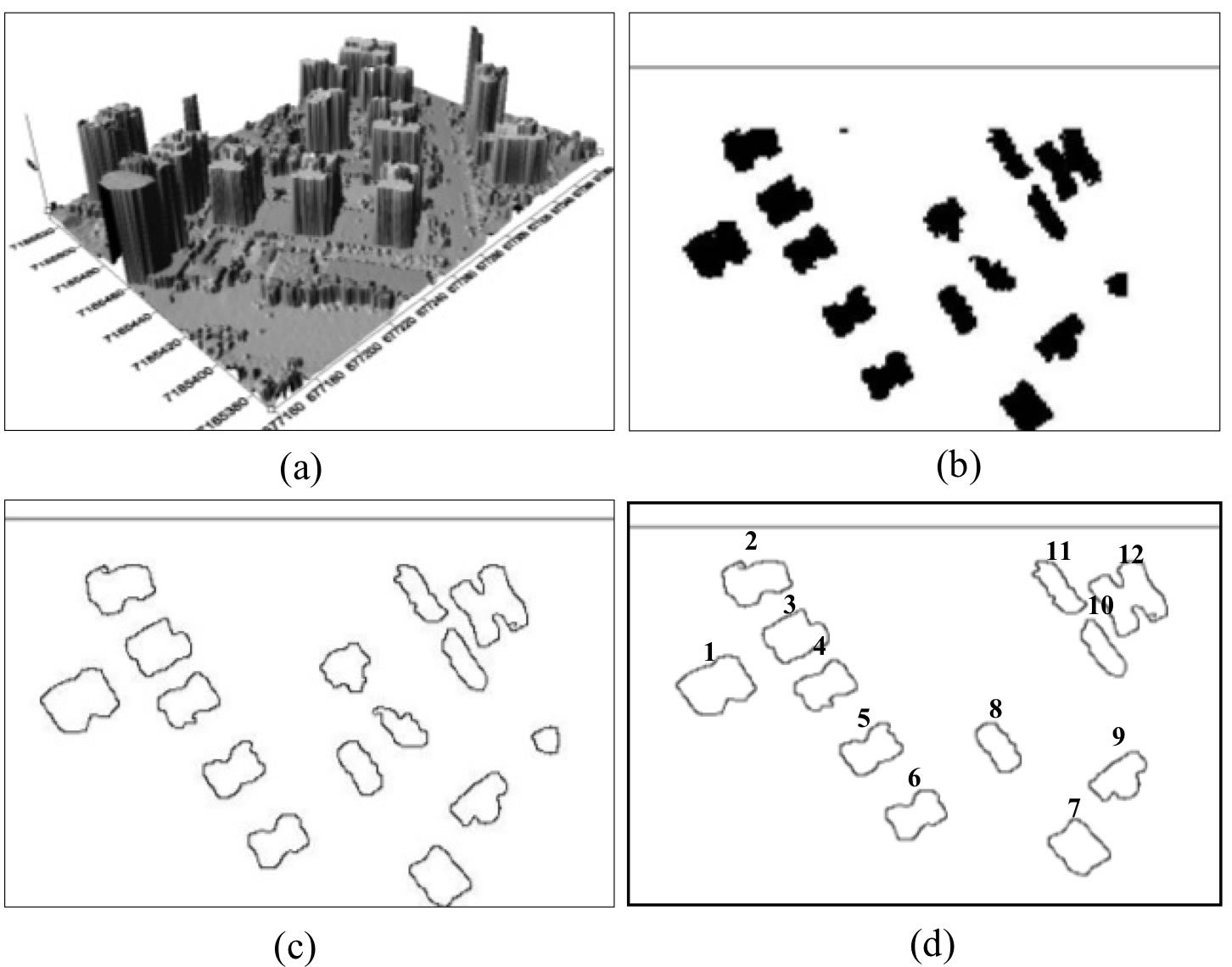
Figure 2 - Results for test areas 2. (a) Three-dimensional visualization of the test area 1 DSM; (b) Aboveground regions; (c) Contours of the aboveground regions; and (d) Identified building roof contours.
In Figure 2(c), the non-building contour is a small and approximately round contour. Although the building roof contours were irregular, the first two main directions were relatively well defined for most contours. Approximately 3 or 4 buildings had small, rounded sides, and therefore, only the primary orientation could be determined with sufficient accuracy. From this discussion, it is expected that the spatial attributes should be the most important elements for determining the correct building contour configuration. Figure 3(d) shows that 12 out of 14 building roof contours were extracted, and the non-building object was eliminated.
The quality parameters derived using test area 1 show that the proposed method performed better with building roof contours 1 (AC1= 92%) and 2 (AC2= 88%). The poorest area completeness (AC3= 62%) was obtained for building roof contour 3. Because one out of four building roof contours was not extracted and no false positives were verified, the of false negatives (#FN) and BER parameters were 1 and 100%, respectively.
As a result using test area 2, FN= 2 and BER= 100%. The quality parameters shows that five building roof contours had ACi values (Ai= 98%, i= 2, 7, 8, 9, 10) that approached the optimal value (100%). Less than ideal results, in terms of area completeness, were obtained for buildings 1, 11, and 12, although all of the ACi values were above 80%. In conclusion, the method performance for this experiment can be considered satisfactory.
4. Conclusion
To evaluate the proposed method, two experiments were conducted, involving varied landscape complexities. In general, the method showed a satisfactory performance, as no false positives occurred and few false negatives were verified. In addition, the area completeness values showed that nearly all of the extracted building roof contours were good approximations of the corresponding reference contours.
As a perspective for this paper, at least one improvement of the energy function was planned. In the present form of the energy function, the separation between buildings and other objects (mainly vegetation) is mainly based on geometric attributes, i.e., the rectangularity and spatial constraints. In order to differentiate better roof and vegetation surface, we will add an energy term of surface smoothness. Another direction for future work is the extension of the method to reconstruct roofs in 3-D.
5. Acknowledgment
The authors would like to thank LACTEC for provided LiDAR data used in our experiments.
6. References
Akçay H G, Aksoy S. "Automatic Detection of Geospatial Objects Using Multiple Hierarchical Segmentations". IEEE Transactions on Geoscience and Remote Sensing, 2008, 46, 7: 2097- 2111.
Ballard D H, Brown C M. Computer Vision. Prentice Hall, Inc., Englewood Cliffs, New Jersey, 523p. 1982.
Cerny V. "Thermodynamics approach to the traveling salesman problem: an efficient simulation algorithm". J Optimization Theory Appl, 1985, 45: 41–51.
Collins N E, Eglese R W, Golden B L. "Simulated Annealing - An Annotated Bibliography". Am. J. Math. Manag. Sci., 1988, 8: 209–307.
Eglese R W. "Simulated annealing: a tool for operational research". Eur J Opl Res. 1990, 46: 271–281.
Ferraioli G. "Multichannel InSAR Building Edge Detection". IEEE Transactions on Geoscience and Remote Sensing, (2010), 48, 3: 1224-1231.
Fua P, Hanson A J. "Resegmentation using generic shape: Locating general cultural objects". Pattern Recognition Letters, 1987, 5: 243-252.
Glover F, Greenberg H J. "Newap proaches for heuristic search: a bilateral linkage with artificial intelligence". Eur J Opl Res, 1989, 39: 119–130.
Jain R, Kasturi R, Schunck B G. Machine vision. MIT Press and McGraw-Hill, Inc New York. 1995.
Jwa Y, Sohn G, Tao V, et al. An implicit geometric regularization of 3d building shape using airborne lidar data. In International Archives of Photogrammetry and Remote Sensing, XXXVI, Beijing, China, 2008, 5. 69–76,
Kirkpatrick S, Gelatt Jr C D, Vecchi M.P. "Optimization by simulated annealing". Science, 1983, 220: 671–680.
Kopparapu S K, Desai U B. Bayesian approach to image interpretation. 127p. 2001.
McCormick G, Powell R S. 'Derivation of near-optimal pump schedules for water distribution by simulated annealing". J Opl Res Soc, 2004, 55: 728–736.
Metropolis N, Rosenbluth A. W, Rosenbluth M N, et al. "Equations of state calculations by fast computing machines". The Journal of Chemical Physics. 1953, 21, 6: 1087–1092.
Müller S, Zaum D W. Robust building detection in aerial images. In The International Archives of thePhotogrammetry, Remote Sensing and Spatial Information Sciences, Vienna, Austria, vol. XXXVI, 2005. 143-148.
Rutenbar R A. "Simulated annealing algorithms: an overview". IEEE Circuits Devices Mag, 1989, 5.
Rüther H, Martine H M, Mtalo E G. Application of snakes and dynamic programming optimization technique in modeling of buildings in informal settlement areas. ISPRS Journal of Photogrammetry and Remote Sensing, 2002, 56: 269-282.
Shutler P M E. "A priority list based heuristic for the job shop problem". J Opl Res Soc, 2003, 54: 571–584.
S?rmaçek B, Ünsalan C. "A Probabilistic Framework to Detect Buildings in Aerial and Satellite Images". IEEE Transactions on Geoscience and Remote Sensing, 2011, 49, 1: 211-221.
Starck V. Implementation of Simulated Annealing optimization method for APLAC circuit simulator. Master´s Thesis, Helsink University of Technology, 1996.
Wang O, Lodha S K, Helmbold D P. A Bayesian Approach to Building Footprint Extraction from Aerial LIDAR Data. Third International Symposium on 3D Data Processing, Visualization, and Transmission, Chapel Hill, USA, 2006, 192 – 199.