
 HOME | ÍNDICE POR TÍTULO | NORMAS PUBLICACIÓN
 Espacios. Vol. 37 (Nº 05) Año 2016. Pág. 6
Claudimar Pereira da VEIGA 1; Cássia Rita Pereira da VEIGA 2; Ubiratã TORTATO 3
Recibido: 04/10/15 • Aprobado: 24/11/2015
4. Effectiveness and Selection of the Forecasting Method
ABSTRACT: In order to achieve competitive advantage in a floating environment the organization needs to make the right decisions, on an adequate time, and based on quality information. In this context, the demand forecasting is the base for strategic and planning decisions on a supply chain, since it provides subsidies for the plans of production, marketing, finances, and human resources. The quality of forecasting has direct influence on the level of service offered to the consumer, as well as in the budget planning of the companies. Due to the strategic importance of the demand forecasting for the organizations, different methods were studied until this moment and are available to be used on varied situations. Therefore, the goal of the article is to describe the fundamental characteristics of a demand forecasting process, and review the main methods, especially those based on time series. The article refers to a review work, synthesizing and expanding the information available on the literature and, in the same time, suggesting areas that weren't approached by researches. The found results suggest that the subject was not exhausted and that is a field to be explored. There is a need of new investigative researches on forecasting due to the process complexity and the applicability in different situations. |
RESUMO: Para alcançar vantagem competitiva em um ambiente de flutuações, a organização deve tomar decisões certas, em tempo adequado e baseado em informações de qualidade. Neste contexto, a previsão da demanda é a base para decisões estratégicas e de planejamento em uma cadeia de suprimentos já que fornece subsídios para os planos de produção, marketing, finanças e recursos humanos. A qualidade da previsão exerce influência direta no nível de serviço oferecido ao consumidor bem como no planejamento orçamentário das empresas. Exatamente devido à importância estratégica da previsão da demanda para as organizações, diversos métodos foram estudados até o momento e estão disponíveis para serem utilizados em situações variadas. Dentro deste contexto, o objetivo deste artigo é descrever as características fundamentais de um processo de previsão de demanda e rever os principais métodos, em especial, os baseados em séries temporais. O artigo se refere a um trabalho de revisão sintetizando e ampliando as informações disponíveis na literatura e, ao mesmo tempo, sugerindo áreas ainda não abordadas pelas pesquisas. Os resultados encontrados sugerem que o assunto ainda não foi esgotado e se mostra um campo a ser explorado. Há necessidade de novas pesquisas investigativas em previsão devido à complexidade do processo e à sua aplicabilidade em situações diversas. |
The forecasting is a subject that assumes increasingly importance for the stakeholders in a competitive market. The limited predictability and the high level of uncertainty are present in different areas important in our lives. An imprecise forecasting proves the disastrous consequences in areas that go from economy, business, climate, medicine [1]. The forecasting has many purposes and strategies, for example, defining budget, establishing sales and marketing quotas, planning of production expenses, production, financing, and controlling the inventory [2-4], as well as the business cycle in an organization [5]. Vieira and Favaretto [6] quote, for example, the importance of the inventory level in a company with limited production capacity. In this context, the more assertive the demand forecasting lower will be the impacts and costs on the productive chain. On the other hand, the increased mistakes can compromise the costs of the supplies chain and the organization competitiveness [1,7,8].
The organizations need, somehow, know how to dimension their productive capacities on a way that they fit with the demands, avoiding waste of time, material, and energy, or the lack of products to serve the final consumer. The forecasting role, among them the demand forecasting, is to provide supplies for the strategic planning of the organization [3, 9, 10]. To achieve competitive advantage in an environment of constant fluctuations, in order to reduce the forecasting mistake, the organization needs to make right decisions, on the right time, and based on quality information. Obtaining an accurate demand forecasting is the critical point of this process [11, 12]. The forecasting tries to calculate and predict a future circumstance providing a better evaluation of the commercial available information. The forecasting always represents a prominent role on the system of decision support. [13].
Van Der Meijden et al.(14) analyzed the forecasting quality about the production and viability of forecasting system. The forecasting quality enables a better operations planning. Quality of forecasting has direct influence on the services offered to the consumer and level of storage. If a forecasting is more accurate and is approved, it means that the production can anticipate better the client's demand. A better forecasting demand can reduce the investments and the inventory since there will be less uncertainly on a future demand [15, 16].
In this context, the goal of this article is to describe the fundamental characteristics of a demand forecasting process, and review the main methods of forecasting that are more common and easier to use, in especial, the ones based on temporal series. Within this purpose, the current work is divided in six sections. The next section describes the methodology. Section three describes the characteristics and steps of a forecasting process. Section four approaches the quantitative methods based on temporal series, and verifies the extension and concepts of the most used and applied models. Section six the work is finished by a conclusion and suggestions for further researches.
The current work has as a goal to describe and review through formulas and analysis the main concepts of demand forecasting and the most common quantitative models used, based on the literature. It is an exploratory study with the use of bibliography and documental research with longitudinal and transversal cutting [17,18]. The theoretic development contemplates the different characteristics and steps of the forecasting process and the most used methods, and also the effectiveness and selection of the preview method.
The forecasting is a probabilistic estimation or description of a value or further condition [19]. The forecasting includes an average, a variation within a limit, and a probabilistic estimation of variation. There are different methods that can be used on forecasting. However, the basic concept is the same: the behavior patterns from the past will continue in the future, in other words, they assume that the sales of a period of a passed time will be the same as the sales of a corresponding period in the future. In fact, almost all of the forecasting methods are based on the main idea that the past will repeat [15,16, 20].
There are certain desirable characteristics on the forecasting process that implicate directly on its use: (i) the forecasts must be done quickly, easily, and with low costs [2, 3]; (ii) the forecasting previews must be clearly listed so they can be followed with a routine [21]; and finally, (iii) the forecasting system must be capable to introduce new information on an easy way and with low costs, manually or by the use of a computational program [11]. This last characteristic is very important to guarantee the forecasting since, intuitively, the historic data can provide a feasible estimate of demand through the forecasting models [13].
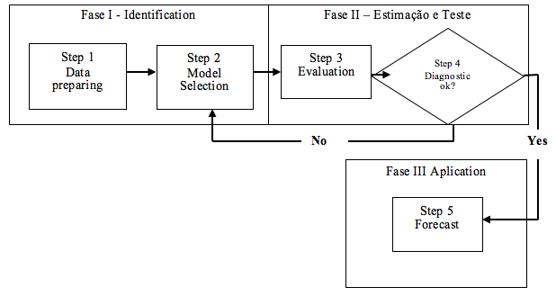
The elaboration and selection of strategic tools for the implementation of a forecasting system requires from the organization the knowledge and ability in four basic areas: (i) identification and definition of problems to be taken care; (ii) the use of forecasting methods; (iii) procedures for the selection of an appropriate method for specific situations; (iv) organizational support to adapt and use the required forecasting methods [22]. The demand forecasting when used as a strategic tool, must consider the following steps: (i) problem definition; (ii) data collection; (iii) pre-analysis of data; (iv) model choice and adjustments; (v) use and continued evaluation of the selected model [21]. DeLurgio [20] quotes that the forecasting process is a statistic-mathematical effort and a scientific method. He describes the forecasting process as a scientific methodology in seven steps, according to the adapted and illustrated on Figure 1.
Figure1: Steps of the scientific forecasting process
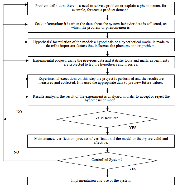
Source: adapted from DeLurdio [20]
Researches have been developed in order to evaluate the performance of scientific methodologies based on the models of preview, but the found results suggest that there still is the need of new investigatory researches due to the complexity of the forecasting preview and the applicability in different situations [23]. The preview process is very complex and requires the adaptation to an appropriate method for each system to be treated. The main quantitative methods will be quickly described here. Qualitative methods, casual methods, simulation methods, and hybrid methods will not be approached on this study.
3.1. Quantitative methods based on temporal series
A temporal series is a selection of numeric data obtained on regular periods of time, in other words, is a set of observations organized in time. For Martinez and Zamprogno [24], a temporal series is a stochastic process that generates observations in the time of a variable y which represents successive measures of an interest phenomenon; These data can suffer influence of some factors such as randomly, tendency, seasonality, scientific pattern, cycle pattern, correlated pattern, or a combination of them.
Martinez and Zamprogno [24] also quote that the main goal of the temporal series analysis is to investigate the generating mechanism of data, describe its behavior using graphics to check the tendency existence, cycles and seasonal variations, for example. In temporal models, the whole observed demand can be divided in a systemic and a random component. From the systematic component is obtained the demand value. It can be divided in: level (current unseasonal demand), tendency (demand tax of increase or decrease for the next period), and seasonality (predictable demand fluctuation) [25].
The random component represents the process part that must be eliminated by the forecasting. The company can only preview the random component in dimension and variables, what allows measuring the forecasting mistake (difference between forecasting demand and real demand). The method performance can be evaluated by the relation between the forecasting mistake and the random component. The models of forecasting must preview the systemic component and estimate the random component [16, 25].
Souto et al.[26] describe four types of temporal series: globally constant series, which presents tendency, series with additive seasonality and series with multiplicative seasonality. The globally constant series do not present tendency, and the series' values float randomly around a fixed amount. A reasonable model for this series is:
![]()
On which Zt represents the series values, μ the values on which they float, and Ԑt the random mistakes. The series that present the tendency estimate the level and tendency values of the series on the instant t through the following equations:
The series with additive seasonality are formed by adding: the level, tendency, a seasonal factor, and a random mistake. The projection of the series future values can be found through the equation:
![]()
on which t is the current period and k = 1 if h<s, k = 2 if s<h<2s. Therefore, in order to calculate the forecasting of the series' future values is necessary to estimate the level and the tendency of the series on the current period and the values of the seasonal factor corresponding to the last period of seasonality. These estimative are found through the following equations:
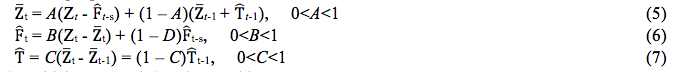
On which A, B, and C and smoothing constants.
The series with multiplicative seasonality and additive tendency are schematically represented, as shown below, for a period s:
![]()
The values projections of the series can be found through the equation:
![]()
For Chopra and Meindl [25], within the temporal series models, there are two basic categories: static and adaptable. In the moment of the static forecasting there isn't an update of the estimative or the systemic component, even facing the changes on the new demands. This category considers the future forecasting mistakes as part of the random component of the demand. In the model of the adaptable forecasting it is made the update of the estimative and the systematical component. This model attributes the forecasting mistake and the wrong estimative of the systematical component and to the random component.
A temporal series can be classified as deterministic or stochastic. It is deterministic when the future values of the series can be established precisely by a mathematical functional relation of the type of the type y = f (time). It is stochastic when the future values can be exposed in probabilistic terms, since the series is described through a functional relation that involves not only time, but also a random variable of the type y = f (time, α), on which α is the residual random time [26]. Following, it will be described methods based on temporal series.
For Makridakis et al. [21], the simple moving averages describes procedures on which for each new available observation, a new average can be calculated. It is not considered the previous periods and the previous observations are substituted by a more recent period. This way, the value of the forecasting will be:
![]()
If an analyzed series presents a lot of randomly or small changes on its pattern, a bigger number of observations can be used on the calculation of a moving average, there is to say that the moving average in this case is more immune to noise and short movements [4]. In case of the series that present low random float on the data or significant changes, the lower number must be used for the size of the observation window, otherwise the forecasted series can react on a very slow way to these significant changes.
For DeLurgio [20] and Veiga et al. [4], this method brings good results only when the demand doesn't show a pattern, in other words, there is no tendency for seasonality. The moving average method presents different limitations and, therefore, the practical application is very restrict. Veiga et al. [11], they quote the SMA method's disadvantages: (i) it can generate cyclical movements; (ii) it is affected by the extreme values; (iii) the older observations have the same importance of the current ones; (iv) the maintenance of a high number of data. The advantages of the SMA method involve simplicity, implementation facility and the possibility of manual processing. Besides, the presentation of this method is valid as a reference for the comparison of the other studied methods development [21].
Usually it is true that the immediate past is more relevant to forecast the immediate future [9]. In this case the recent values must receive a better ponderation on the moving average, as quoted by Pindyck and Rubinfeld [27]. The Weighted Moving Average is a variable of the SMA model. The goal of this method is to check more weight to the more recent data, and less to the old ones. An advantage of this method is that the weights that are attributed to the past demands can vary. However, the determination of the great value can be expensive. Besides, this method does not consider the seasonality and tendency, and requires the maintenance of a big number of data [11].
The calculation of the WMA involves the multiplication of each one of the data for a different weight. There are two methodologies; one uses a fixed weighting factor, the other uses a variable. In general, the moving average on the k-th weighted poking can be described by the equation:
![]()
Based on the literature, the Exponential Smoothing method, the new forecast is simply the old forecast with an adjustment for the mistake that happened on the last preview [21]. The model of SES has easy application because requires only three data: (i) more recent preview; (ii) more recent data; and (iii) a constant smoothing [20]. The smoothing constant (α) determines the weight given to the more recent past observation, and controls the tax of smoothing or average. This constant is between 0 to 1, that is to say, 0 < α < 1.
By this method, we can express the level in a certain period with a function between the current demand and the level on the past period, according to the equation below:
![]()
On which Lt+1 = the estimative of the final period t+1, Dt+1 = real observed demand on the period t+1 and α = smoothing constant for the level. A way to estimate the SES consists in supposing that this constant must be a weighted average of the previous values of the series, on which the weights exponentially decrease as the time of observation gets more distant from the present [26]. Mathematically we have:
![]()
On which ![]() t, is called the exponential smoothed value, and α is the smoothing constant. The lower the value of α, lower will be the influence of more recent values on the forecasting.
t, is called the exponential smoothed value, and α is the smoothing constant. The lower the value of α, lower will be the influence of more recent values on the forecasting.
The value of the constant α can be chosen. According to Downing [28], it must be chosen the value that generates better forecasting. If α is considered equal to 1, it means that the estimated value will be equal to the one achieved on the last period, and the past values will not be considered. If α is considered equal to zero, it means that the forecast will be equal to the last estimated value. If α is between 0 and 1, it will be a balanced situation between the two extremes [28]. The chosen value for Soares et al. [29] must minimize the squared errors addition (SEA). Therefore, α must be between the values of the series Zn1 and Zn2, as shown below:
![]()
Martinez and Zamprogno [24] describe that a reasonable way of choose α is through the visual inspection, in other words, if the series develops on a smooth way it makes sense to use a high value for α, since the series develops erratically it is reasonable to attribute lower weight to the last observation. They also suggest that a more objective method would be to choose the value of α that minimize the addition of the errors squares on the forecast a step ahead.
Around 25 years ago, the SES methods were considered a grouping of techniques for the extrapolation of many types of univariate temporal series. However this method has been deeply used in business and industries, they, on the occasion, didn't receive much attention of the statistician and didn't have a well developed statistical base. Gooijer and Hyndman [30] show the historical evolution of these methods.
Snyder at al. [31] show that the methods that use SES are frequently used to control the inventory. These authors use the SES model with simple source of error for demand forecasting. They suggest that the chosen methodology has four advantages on the others: (i) the use of algorithm can be avoided when the variance is not stationary; (ii) the more common types of tendency and seasonality can be modeled; (iii) the models are easily understandable if the components, tendency, and seasonality levels are explicit; and (iv) this method can be used in many models. Snyder et al. [31] also used the SES method to forecast the demand's lead time for the inventory control. This study showed the opportunity of methods implementation that ensures the storage secure adjustment when changing the tendency and seasonality. Summarizing, the SES model is a simple and pragmatic approximation for the punctual forecasts that are based in weighted exponential averages from the past forecasts observation. He SES method development when applied to different series increases the applicability in researches that involve sales preview [32].
Until the 60's decade, the exponentially weighted average moving method (EWAM) was widely used. A research held by Holt in 1957 extended concepts of EWAM adding the tendency component to the forecasting process [33]. According to DeLurgio [20], the advantage of the Holt method is the flexibility on which the level and the tendency can be smoothed with different weights. This author shows, also, that the Holt method requires that two parameters are optimized. Considering that the research for the better parameters combination is more complex that for a simple parameter, the disadvantage of the Holt method is the limitation for the data with seasonality [34].
On the Holt method, the estimative of level and tendency is the weighted average between the observed value and the old estimative, according to the equation shown below:
![]()
On which Lt = estimative of tendency on the end of the period t, Tt+1 = estimative to the tendency on the end of period t+1, Dt+1 = real demand observed on the period t+1, α = smoothing constant for the level, β = smoothing constant for the tendency. The objective choice of the α and β values is by the minimization of the forecast errors square addition a step ahead [24].
The Holt-Winters model (HW) was developed in the 60's decade during the evaluation of forecast accuracy held by the Holt method [33]. These studies added a seasonality component on the forecasting process. On the development of the HW model, there was an expansion of the EWAM method formula, adding many components in various combinations: seasonal multiplicative, seasonal additive, multiplicative with tendency, and additive with tendency. The new program was easy, quick to compute, required low storage of data, offered less weight to old data, and presented robustness parameters [33].
Pellegrini and Fogliatto [22] also classified the model HW in two groups: additive and multiplicative. On the additive model, the difference between the higher and lower demand value in the stations remains relatively constant, that is to say, the amplitude of the seasonal variation does not change as the time passes. On the multiplicative model, the amplitude of the seasonal variation increases due to the time [33].
The multiplicative model of HW is used on the seasonal data model on which the amplitude of the seasonal cycle increases due the time. It can be represented by:
![]()
on which b1 is the permanent component (of average), b2 is a linear component of tendency, ct is a multiplicative seasonal factor, and et represents the random error, independent, and identically distributed. The use of this model requires the previous knowledge of the seasonal cycle duration existing on the temporal series, regarding the time unity on which the data are collected. Therefore, if a series presents annual seasonality with monthly collected data, the seasonal cycle will be L = 12 months. The relation existing between the seasonal factors and the cycle duration is:
![]()
The multiplicative seasonal model can also be applied on series on which the linear tendency is not checked; therefore, resets the component of tendency b2. The use of the multiplicative model demands the estimative of initial values (on time t = 0) for the parameters b1, b2 and ct. These estimators are identified by ![]() 1(0),
1(0), ![]() 2 (0) and
2 (0) and ![]() t(0), t = 1, 2,..,L, with estimative represented by
t(0), t = 1, 2,..,L, with estimative represented by ![]() 1(0),
1(0), ![]() 2(0) and
2(0) and ![]() t(0). Different estimators are available on the literature [11].
t(0). Different estimators are available on the literature [11].
For Souto et al. [26], the series with additive seasonality are formed by the addition of: level, tendency, a seasonal factor, and a random error. The future values projection of the series can be found through the equation:
![]()
n which is the current periods and k = 1 if h<s, k = 2 if s<h<2s. Therefore, in order to calculate the future values previous of the series is necessary to estimate the level and the tendency of the series on the current period and the values of the seasonal factor corresponding to the last period of seasonality. These estimative are found through the following equations:
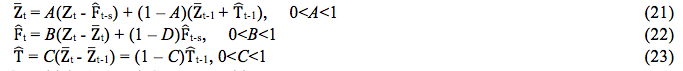
On which A, B and C are smoothing constants.
The series with multiplicative seasonality and additive tendency are schematically represented are shown below for a period s:
![]()
The projections of the series future values are found through the equation:
![]()
The Winter model requires the use of computational packages based on interactive procedures. According to [20] the use of the HW model is popular in some commercial systems of forecast due to the advantages that offer, such as: easy interpretation of the seasonality indexes and management knowledge, great applicability, it is more intuitive, and can be suitable to efficient computational algorithms. However, the HW method can became really complex for the data that do not have identified tendency and seasonality [35].
On the HW method, the reviewed estimative of level, tendency, or seasonality factor is the weighted average and the observed value, and the old estimative, according to the following equations:

On which Lt = level tendency estimative by the end of the period t, Lt+1 = level estimative by the end of the period t+1, Tt = tendency estimative by the end of the period t, Tt+1 = tendency estimative by the end of period t+1, St+1 = seasonality factor estimative for the period t+1, St+p+1 = seasonality factor estimative for period t+p+1, Dt+1 = real demand observed on period t+1, α = smoothing constant for the level, β = smoothing constant for the tendency, γ = smoothing constant for the seasonality.
For Souto et al. [26], the smoothing constant must be chosen by the minimization criteria of the square addition of the errors that produce the lower sum of the residues squares of the step ahead forecasts. The HW method is a sophisticated extension of the sophisticated exponential smoothing methodology. For Segura and Vercher [36], the HW model is simple and can supply precise forecasting results such as the ones obtained with the more complex techniques. The components of this model are obtained by the fixation of the constant values α, β and γ to estimate the initial values and stabilize specific values for the parameters.
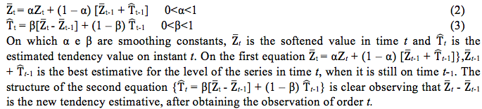
For Souto et al. [26], the HW model proposal is to estimate the level values and the tendency of the series in the instant t through the following equations:
![]()
On which α and β are smoothing constants, ![]() t is the smooth value in time t and
t is the smooth value in time t and ![]() t is the estimated value of the tendency on instant t. On the first equation {
t is the estimated value of the tendency on instant t. On the first equation {![]() t = αZt + (1 – α)[
t = αZt + (1 – α)[![]() t-1 +
t-1 + ![]() t-1]},
t-1]},![]() t-1 +
t-1 + ![]() t-1 is the better estimative for the series level in time t, when it still is in time t-1. The structure of the second equation {
t-1 is the better estimative for the series level in time t, when it still is in time t-1. The structure of the second equation {![]() t = β[
t = β[![]() t -
t - ![]() t-1] + (1 – β)
t-1] + (1 – β)![]() t-1} it is clear when observed that
t-1} it is clear when observed that ![]() t -
t - ![]() t-1 is the new estimative of the tendency, after obtaining the observation of t.
t-1 is the new estimative of the tendency, after obtaining the observation of t.
In order to use the equations above, it is necessary the values of the initials. It is used ![]() 2 = Z2 and
2 = Z2 and ![]() 2=Z2–Z1.The forecasts are made through the following equation:
2=Z2–Z1.The forecasts are made through the following equation:
![]()
On which ![]() t(h) represents the observation forecast of t + h in time t.
t(h) represents the observation forecast of t + h in time t.
The autoregressive integrated moving average model (ARIMA) represent an important class in the stochastic methods used in stationary temporal series. They assume that the process is still balanced on the constant average level. An extremely used model on the temporal series representation is the autoregressive model [37]. For Pellegrini and Fogliatto [22], the ARIMA models are built based on the autocorrelation when is possible to identify the existence of correlation among the observations. With seasonal demand data repeat a cycle pattern of variation during the time, the supposition of autocorrelation is, as a general rule, valid. For Zhang [38] and Medeiros et al. [39], the Box-Jenkins methodology includes three interactive steps: (i) model identification; (ii) parameters estimation; and (iii) checking diagnostic.
The identification and data transformation it is frequently necessary in order to turn the stationary temporal series. Stationary is a necessary condition when building the ARIMA model [11]. The stationary temporal series keeps the property and its statistics characteristics, such as the meaning and structure of autocorrelation constant in time. When the temporal series present tendency or seasonality, the data must be treated in order to remove these characteristics and stabilize the variance before applying ARIMA model. In order to achieve stationary data, Makridakis et al.[21] and DeLurgio [20] suggest the use of the following procedures: (i) data projection of the series in graphics to verify the existence of a pattern; (ii) mathematical transformation in the series data to stabilize the variance; (iii) using the autocorrelation function (ACF) and the partial autocorrelation function (PACF) to verify the existence of a pattern on the series data; (iv) using the differences of the data to obtain stationarity. Once the model is specified, the parameters estimation is directed. The parameters are estimated by minimized errors measures. That can be done with nonlinear optimization. To select the more adequate model it is recommended the use of specialized software [4].
Based on Figure 2, the last step on building the ARIMA model is the diagnostic of adequacy checking. If the model is not the adequate one, a new model must be tested following steps 1 and 2 again. The diagnostic information can help on the alternative model suggestion. For Medeiros et al. [39], the following aspects must be considered: (i) statistical significance of the coefficients; (ii) analysis of the ACF and PACF, in order to verify if there is any orientation of the purely AR or MA models; (iii) verify if there could be more than one plausible model to determine which one has the lower sum of square errors; and (iv) residues analysis, to discard the consideration of other patterns. The previous process is presented on Figure 2.
Figure 2: Schematic representation of ARIMA methodology to model the temporal series.
Source: Adapted from Makridakis et al. [21] and DeLurgio [20]
The Box-Jenkins models are divided in autoregressive (AR), and moving average (MA). The autoregressive models (AR) explore the autocorrelation of the data generator process, in other words, the correlation existing between a temporal series. The moving average models explore the autocorrelation structure of the forecasting errors, in other words, the correlation existing between the successive errors. Models that explore simultaneously the autocorrelation structure of the data generator process and the forecast errors are called moving average and autoregressive, and designated ARMA.
For Martinez and Zamprogno [24], the autoregressive model of order p, denoted by AR(p) can be defined as:
![]()
on which ut ~ RB (0,σ2) is the White noise, ϕ1, ... ϕp are the autoregressive parameters and c is a parameter that allows the process to have an average different from zero. The most used notation is:
![]()
Another known model in this methodology is the called moving average process of order q, denoted by a MAq, which is on the form:
![]()
on which ut ~ RB (0,σ2). The usual notation to describe this process is:
![]()
on which θ(B) = 1 + θ1B + ... + θqBq. Generally, the process can be defined autoregressive of moving average ARMA (p,q) this way:
![]()
on which ut ~ RB (0,σ2), 0s ϕ's and theθ's are the autoregressive parameters and moving average respectively, or yet ϕ(B)yt = c + θ(B)ut, on which ϕ(B) and θ(B) are the polynomials AR and MA usual and the stationarity conditions regarding the AR process and the inverted situation regarding MA remain. If the series is not stationary, the process can be integrated in order d, that is to say, yt is not stationary, but the difference of order d is stationary. There is an ARIMA process (p,d,q) defined as:
![]()
With the goal of considering the seasonal movements, the class of ARIMA models was extended In many occasions it is not possible to transform yt + to remove the seasonality, that is to say, the seasonality can present a dynamic pattern. That means that it is necessary to consider a stochastic seasonal component in a model in order to adjust to the original series. The new ARIMA model is known as seasonal ARIMA, or SARIMA. So yt is the observed interest series and s periods by year:
![]()
on which the seasonal autoregressive with order P, stationary, is:
Θ(Bs) = 1 – Θ1Bs - ... – ΘQBsQ, ![]() = (1 – Bs)D, on which D indicates the number of "seasonaldifferences". The class of multiplicative seasonal models (p,d,q) x (P,D,Q) is given by: the average operator of seasonal moving media of order Q, invertible,
= (1 – Bs)D, on which D indicates the number of "seasonaldifferences". The class of multiplicative seasonal models (p,d,q) x (P,D,Q) is given by: the average operator of seasonal moving media of order Q, invertible,

![]()
It can be supposed that it is possible to combine the ARMA model with a regression structure of the form:
![]()
on which yt is the variable, Zt is the independent variable, Ԑt + is a white noise is α, ϕi,θj are the unknown parameter. The model above is known as ARMAX and it can be extended to include more than one explicative variable (hexogen). This model is used on the forecast of the electricity prices market by Arciniegas and Rueda [40]. The Box-Jenkins models are more complex, and require the use of dedicated computational package, not available in the market until recently [11].
The artificial neural networks (ANNs) are mathematical models inspired on the organization and functioning of the biologic neurons [41]. There are numerous variations of ANNs that are directly related to specific tasks. A ANNs is basically a set of inter-connected elements called neurons, that are distributed in three zones: entrance neurons, intermediary neurons, and exit neurons. The neurons are interconnected and interact with the goal to achieve a desirable behavior for a system. Each neuron receives the status of the entrance and, through a function applied to the weight vector, produces a signal (exit), which is taken by the following neuron. The ANNs adapt to an environment according to a training that consists in searching the relevance of the connections that codify the knowledge that the system must acquire [42]. In order to determine completely the structure, the ANNs need an inter-connection architecture, activation functions that measure the importance of a data, costs function that evaluate the network exit, and a training algorithm to optimize the costs function [24].

The ANNs methodology is more efficient on not linear the temporal series preview, treating the forecasting issue as an approximation problem. For Calôba et al. [43] and Zhang [38], in any problem to be solved through the use of neural nets, it is necessary the use of entrance-exit pairs already known. Many times the quantity of available pairs is not too big, and yet the data must be separated in two well defined sets, the training set and the test set.
The network training is done using a training set. It is, however, necessary to measure the network performance, considering how it responds to entrance-exit pairs, not presented during the training (test set). This is important because an extended training can bring a problem known as overtraining, that can lead to a super specialization of the network (mainly when there aren't a lot of data) and a loss of network capacity to respond well to never presented data (loss of capacity generalization). It is virtually accept that the best network is the one that supplies the smaller error in the validation set and the minimum error for the test set [44]. The validation set corresponds to the entrance-exit pairs, that are not presented to the network during a training and are not parameters to close the training, that is to say that they represent a totally new set to be presented to the network for development evaluation.
According to Calôba et al. [43] and Zhang [38], the neural networks get highlighted efficiency when they are not linear. The first ones make three important propositions: (i) neural network are not always the best solution. Many times, when a new forecasting technique or optimization appear with interesting results, and this becomes quickly the "best" existing technique; (ii) the non-linearity is a problem that can be treated by neural networks; (iii) associating classic linear methods and neural networks seems to bring good results on the treatment of non-linear problems. The most known and tried neural network is the feedforward type [38]. On this model, the neurons are disposed in layers, usually two active layers. The neurons of a layer only connect to the ones on the following layer. Three types of layers can be highlighted on the structure of a network of this gender. The first layer, or "entrance layer", is not composed by neurons, but simply by the entrance signals. The following layer, known as "intermediary layer" or "hidden layer", is composed by N neurons, and makes some transformations. By the end, there is a layer known as "exit layer". There are many neurons on this layer when the number of desired, each exit representing a variable that desires to forecast [44].
The entrance and exit relation (yt) and the entrances (yt-1, yt-2, ..., yt-p) have to follow the mathematical representation:
![]()
On which αj (j = 0, 1, 2,…, q) and βij (i = 0, 1, 2,..., q) are the model parameters frequently called connection weight; p is the number of entrance and q is the number of hidden layers. The logistic function is frequently used as a hidden layer of the transferring function, which is:
![]()
Once the neural network models analyses the past non-linear observation performance (yt-1, yt-2, ..., yt-p), the future value of yt will be:
![]()
on which w is a vector of all the parameters and f is a function determined by the network structure and the connection weights. The choice of the q hidden layers number depends on the data and there is not a systemic role on the decision of this parameter.
Maybe the most important parameter to be estimated in neural networks is the number of the out of phase observations p on the entrance vector dimension. This parameters represents a main role on the structure determination of autocorrelation (non-linear) of the temporal series. However, there is not a theory that can be used to help on the p selection. The next section will approach the effectiveness and the selection of the forecasting method. The next section describes how to choose a forecasting method among the ones previously described.
In order to choose a forecasting method for a data temporal series, it can appeal to some statistic information available that determine the adequate method for a particular situation. Among the criteria that define the effectiveness and selection of a forecasting method selection, it can be quoted [45, 46].
a) Mean square error (MSE): is the average of the forecast square errors. The mean square error estimated the variation of the forecasting error. It is not easily interpreted by itself, and normally compared to other statistic methods. Other limitation would be the fact that the MSE is inappropriate for comparison among series since it regards a depending scale method [30]. Mathematically it can be expressed:
![]()
b) The mean absolute percentage error (MAPE) is the mean absolute error as a percentage of the demand. This method presents problems when the series have closed values for (or equal to) zero. These problems can be avoided including in the analysis only data with positive values; however, this artificial solution limits the method application in many situations [20]. Gooijer and Hyndman [30] show that the MAPE presents the disadvantage of using heavy penalty about positive errors regarding the negative errors. Besides that, these authors also show that more scientific works and discussions are still necessary regarding the symmetric measures proposed up to this moment. Lewis [45] describes that, in practice, a MAPE value lower than 10% can suggest potentially good forecasts. Mathematically, MAPE can be expressed:

c) Mean absolute deviation (MAD): estimate the random pattern deviation, when normally distributed. Also, it is not easily interpreted by itself, being normally compared to other statistic methods. As it happens on the deviation patter, the MAD is not particularly a intuitive patter and it can be easily interpreted on the normal distribution context of the data. DeLurgio [20] shows that for the normal distribution the MAD is the pattern deviation are equivalent measures of dispersion, so the MAD represents, approximately, 80% of the pattern deviation. Mathematically it can be expressed:
![]()
d) Bias: the bias and the reason of bias evaluate the occurrence of overestimation or underestimation of the demand. The forecast bias is the simple sum of the forecast errors. If the forecast errors are originating exclusively from the random components of the forecast, the bias value must vary around zero. If the forecast model does not receive the entire systemic component, the bias value will be different from zero. Mathematically it can be expressed:
![]()
e) Bias Reason (TS - Trecking Signal): it is mathematically the quotient between the forecast bias and the MAD. Chopra and Meindl [25] determine that the bias reason value must be between -6 and 6 to be tolerable. The positive values above 6 detect overestimation of results, and negative values under -6 indicate underestimation of forecast. DeLurdio [20] shows that the TS statistically detects cumulative errors. There are many studied TS techniques until this moment with the need of using them on specific situations. It can be mathematically expressed by:
![]()
According to Slack et al. [47], on the forecast model choice, it must be considered aspects such as the forecast horizon, data availability, necessary precision, and resource availability. Higuchi [48] shows that the use of only qualitative models can not be the best choice since it is impossible to have a numeric dimensioning. The qualitative and quantitative models integration is the best option for an accurate forecast.
Many studies aim to determine the demand forecast development through different criteria [23]. It can be quoted, for example, Lawrance and O'Connor [49] on which the forecast development was determine by the accuracy, propensity, and efficiency. Winklholfer and Diamantopoulos [50] showed that the effectiveness of the forecast is influenced by the short term accuracy, overestimation, and temporality. Armstrong at al. [46] describe that the buying intention contributes to the accuracy of the sales forecast.
This article had as a goal to describe and review through bibliographic, documental, formulas, and applications, the main concepts of the demand forecast and the quantitative methods more commonly used, as well as the main characteristics of a demand forecast process, and review the main methods based in temporal series, normally found and easily implemented in electronic spreadsheets.
On the forecast technique implementations, the companies find out that the forecast is much more complex than a simple project or a selection of an appropriate algorithm and involves the choice of relevant information pieces, information system project, control of data quality, and the definition of management process [51, 52]. Besides, the choice of the appropriate level of complexity depends on the decision making process that the forecast hopes to support. That represents a critical problem about the implementation and adoption of forecast techniques. Many strategic and operational decisions are based on the demand forecast. The demand forecast has been deeply studied by researchers for many decades. Many articles share a common fact: they explore the adoption of forecast qualitative or quantitative methods propose new techniques, evaluate the development of those that already exist and show the complexity of demand forecast in many segments.
There are many methods that can be used in forecasting, however, the basic supposition of the majority is the same: the past behavior will repeat. In general, the more convenient forecast models are parsimonious, that is to say that those with a few parameters and tend to supply more precise previews. However, none of the forecast models can be considered universally the best, indiscriminate the specific situations of the forecast process.
Many studies about the demand forecasting were published until this moment, involving many market segments. Besides that, many questions are still with no answers by the scientific researches. Considering that, there is an importance of the forecast on the strategic planning of the organizations; this study is still stimulating many scientific works in Brazilian universities and in the world. The found results, until this moment, suggest that there is still the need of new investigative studies to the complexity of the forecast process and the applicability in different situations.
[1] S. Makridakis and N. Taleb, "Decision making and planning under low levels of predictability", International Journal of Forecasting, vol. 25, pp. 716-733, 2009.
[2] P. R. Winters, "Forecasting sales by exponentially weighted moving averages". Management Science, vol. 6, pp. 324– 342, 1960.
[3] J. S. Armstrong, "Principles of Forecasting: A Handbook for Researchers and Practitioners". Kluwer Academic Publishers, 2001.
[4] C. P. Veiga, C. R. P. Veiga, A. Catapan, U. Tortato, and W. V. Silva, "Previsão de demanda no varejo alimentício como ferramenta estratégica de sustentabilidade em uma pequena empresa brasileira", Future Sudies Research Journal: Trends and Strategies, vol. 5, no. 2, pp. 113-133, 2013
[5] L. Ferrara, and D. V. Dijk, "Forecasting the Business Cycle". International Journal of Forecasting, vol. 30, pp. 517-519, 2014.
[6] G. E. Vieira and F. Favaretto, "A new and practical heuristic for Master Production Scheduling creation", International Journal of Production Research, vol. 44, n. 18-19, pp. 3607-3625, 2006.
[7] J. S. Armstrong, "Findings from evidence-based forecasting: Methods for reducing forecast error", International Journal of Forecasting , vol. 22, pp. 583-598, 2006.
[8] J. R. Pérez-Gallardo, B. Hernández-Vera, C. G. M. Sánchez, et al., "Methodology for Supply Chain Integration: A Case Study in the Artisan Industry of Footwear," Mathematical Problems in Engineering, vol. 2014, Article ID 508314, 15 pages, 2014. doi: 10.1155/2014/508314.
[9] S. Makridakis, S, Forecasting: its role and value for planning and strategy. International jornal of forecasting, vol. 12, pp. 513-537, 1996.
[10] D. F. Tubino, Manual de Planejamento e Controle da Produção, São Paulo, SP: Atlas, 2000. 220p.
[11] C. P. Veiga, C. R. P. Veiga, G. E. Vieira, and U. Tortato, "Impacto financeiro dos erros de previsão: um estudo comparativo entre modelos de previsão lineares e redes neurais aplicados na gestão empresarial", Produção Online, vol. 12, no. 3, pp. 629-656, jul./set. 2012.
[12] C. Jiang, J. Zhang, and F. Song, "Selecting Single Model in Combination Forecasting Based on Cointegration Test and Encompassing Test," The Scientific World Journal, vol. 2014, Article ID 621917, 8 pages, 2014. doi:10.1155/2014/621917
[13] R. J. Kuo and K. C. Xue, "Fuzzy neural networks with application to sales forecasting". Fuzzy Sets and Systems, vol. 108, pp. 123-143, 1999.
[14] L. H. V. D. Meijden, J. A. E. E. V. Nunen, and A. Ramondt, A, "Forecasting – bridging the gap between sales and manufacturing". International Journal Production Economics, vol. 37, pp. 101-114, 1994.
[15] W. Ascher, "Forecasting: An Appraisal for Policy Makers and Planners". Baltimore: Johns Hopkins University Press, 1978.
[16] P. A. Morettin and C. M. Toloi, "Previsão de series temporais". 2. ed. São Paulo: Atual Editora, 1987. 436p.
[17] R. Yin, "Case study research: design and methods". Beverly Hills: Sage Publications, 1987.
[18] A. C. Gil, "Como elaborar projetos de pesquisa". 4. ed. São Paulo: Atlas, 2002, 175p.
[19] F. Petropoulos, S. Makridakis, V. Assimakopoulos, and K. Nikolopoulos, "Horses for Courses" in demand forecasting, European Journal of Operational Research, doi:http://dx.doi.org/10.1016/j.ejor.2014.02.036, 2014.
[20] S. A. Delurgio, "Forecasting Principles and Applications", Boston: Irwin McGraw-Hill, 1998. 802 p.
[21] S. Makridakis, S. Wheelwright, and R. J. Hyndan, "Forecasting: methods and applications", 3. ed. New York: John Wiley and Sons, 1998. 642p.
[22] F. R. Pellegrini and F. S. Fogliatto, "Estudo comparativo entre os modelos de Winters e de Box-Jenkins para previsão de demanda sazonal", Produto e Produção, vol. 4, pp. 72-85, 2000.
[23] D. Orrell and P. McSharry, "System economics: Over-coming the pitfalls of forecasting models via a multidisci-plinary approach", International Journal of Forecasting, vol. 25, no. 4, pp. 734–743, 2009.
[24] R. O. Martinez and B. Zamprogno, "Comparação de algumas técnicas de previsão em análise de séries temporais", Revista Colombiana de Estatística, vol. 26, no. 2, pp. 129-157, 2003.
[25] S. Chopra and P. Meindl, "Gerenciamento da Cadeia de Suprimentos: Estratégia, Planejamento e Operações". 3. ed. São Paulo: Pearson Prentice Hall, 2001. 465 p.
[26] D. P. Souto, R. A. Baldeón, and S. L. Russo, "Estudo dos modelos exponenciais na previsão", Sistemas e Informática, vol. 9, no. 1, pp. 97-103, 2006.
[27] R. S. Pindyck and D. L. Rubinfeld, "Econometria modelos & previsões". 4. ed. Rio de Janeiro: Elsevier, 2004. 726p.
[28] D. Downing, J. Clark, "Estatística Aplicada", São Paulo: Saraiva, 1998. 455p.
[29] J. F. Soares, A. A. Farias, and C. C. Cesar, "Introdução à estatística". Rio de Janeiro: Guanabara, 1991.
[30] J. G. Gooijer and R. J. Hyndman, "25 years of time series forecasting", International Journal of Forecasting, vol. 22, pp. 443-473, 2006.
[31] R. D. Snyder, A. B. Koehler, and J. K. Ord, "Forecasting for inventory control with exponential smoothing". International Journal of Forecasting, vol. 18, pp. 5-18, 2002.
[32] J. W. Taylor, "Forecasting daily supermarket sales using exponentially weighted quantile regression". European Journal of Operational Research, vol. 178, no. 1, pp. 154-167, 2007. Doi: 10.1016/j.ejor.2006.02.006
[33] C. C. Holt, "Author's retrospective on "Forecasting seasonal and trends by exponentially weighted moving averages", International journal of forecasting, vol. 20, pp. 11-13, 2004.
[34] R. J. Hyndman, A. B. Koehler, J. K. Ord, and R. D. Snyder, "Forecasting with exponential smoothing: the state space approach". Germany: Springer, 2008, 351p.
[35] G. P. Souza, R. W. Samohyl, and R. G. Miranda, "Métodos simplificados de
previsão empresarial", Rio de Janeiro: Editora Ciência Moderna, 2008, 180p.
[36] J. V. Segura and E. Vercher, "A spreadsheet modeling approach to the Holt-Winters optimal forecasting", European Journal of Operational Research, vol. 131, pp. 375-388, 2001.
[37]. G. E. P. Box, G. M. Jenkins, and G. C. Reinesl, "Time series analysis: forecasting and control". 3. ed. Englewood Cliffs, New Jersey: Prince-Hall, 1994, 598p.
[38] G. P. Zhang, "Time series forecasting using a hybrid ARIMA and neural network model. Neurocomputing", vol. 50, pp. 159-175, 2003.
[39] A. L. Medeiros, et al, "Modelagem ARIMA na previsão do preço da arroba do boi gordo". Trabalho apresentado no XLIV Congresso da SOBER, Fortaleza, 2006.
[40] A. I. Arciniegas, I. E. A. Rueda, "Forecasting short-term Power in the Ontario Eletricity Market (OEM) with a fuzzy logic based inference system", Utilities Policy, vol. 16, pp. 39-48, 2008.
[41] S. Haykin, "Neural Networks: A Comprehensive Foundation", Prentice
Hall, 1999.
[42] C. Granger, "Modeling nonlinear relationships between extended-memory variables.
Econometrica". vol. 63, no. 2, pp. 265-279, 1995.
[43] G. M. Calôba, L. P. Calôba, and E. Saliby, "Cooperação entre redes neurais artificiais e técnicas clássicas para previsão da demanda de uma série de vendas de cerveja na Austrália. Pesquisa Operacional", vol. 22, no. 3, pp. 345-358, 2002.
[44] S. Haykin, "Redes neurais: princípios e prática". 2. ed. Porto Alegre: Bookman, 2001.
[45] C. D. Lewis, "Demand Forecasting and Inventory Control". New York: Wiley, 1997. 157p.
[46] J. S. Armstrong, V. G. Morwitz, and V. Kumar, "Sales forecasts existing consumer products and services: do purchase intentions contribute to accuracy?" International Journal of forecasting, v. 16, pp. 383-397, 2000
[47] N. Slack, S. Chambers, R. Johnston, "Administração da Produção". 2. ed. São Paulo, SP: Atlas, 2002. 747 p.
[48] A. K. Higuchi, "A previsão de demanda de produtos alimentícios perecíveis: três estudos de caso". Revista Eletrônica de Administração, vol. 8, n. 1, pp. 1-15, 2006.
[49] M. Lawrence, M. O'connor, "Sales forecasting updates: how good are they in practice. International Journal of Forecasting", vol. 16, pp. 369-382, 2000.
[50] H, M. Winklholfer, and A. Diamantopoulos, "Managerial evaluation of sales forecasting effectiveness: a MIMIC modeling approach". International Journal of Research in Marketing, vol. 19, pp. 151-166, 2002.
[51] Da Veiga, C.P.; Da Veiga, C.R.P.; Del Corso, J.M.; Da Silva, W.V. Dengue Vaccines: A Perspective from the Point of View of Intellectual Property. Int. J. Environ. Res. Public Health, vol. 19, pp. 9454-9474, 2015.
[52] Veiga, C.P; Veiga, C.R.P., Catapan, Anderson ; Tortato, Ubiratã ; Silva, Wesley Vieira . Demand forecasting in food retail: a comparison between the Holt-Winters and ARIMA models. WSEAS Transactions on Business and Economics, vol. 11, pp. 608-614, 2014.
1. Pontifical Catholic University of Paraná - PUCPR and Federal University of Paraná - UFPR – Brasil – claudimar.veiga@gmail.com
2. Pontifical Catholic University of Paraná – Brasil – cassia.veig@gmail.com
3. Pontifical Catholic University of Paraná – PUCPR – ubirata.tortato@pucpr.br