
 HOME | ÍNDICE POR TÍTULO | NORMAS PUBLICACIÓN
 Espacios. Vol. 37 (Nº 24) Año 2016. Pág. 10
Adolfo SACHSIDA 1; Mario Jorge Cardoso de MENDONÇA 2; Tito Belchior Silva MOREIRA 3; Paulo Roberto Amorim LOUREIRO 4
Recibido: 14/04/16 • Aprobado: 12/05/2016
3. Data Base and Evolution of Criminality
RESUMO: The main objective of this study is to analyze the effect of crime repression policies on the homicide rate in Brazil. Two main types of crime repression policies can be highlighted: policies of incapacitation and policies of detention. In terms of public policies, the incapacitation policies are translated as a higher incarceration rate and the detention policies as higher police officers rate. In general, our results prove that putting more criminals away and increasing the number of police officers are valid strategies to reduce the homicide rate, regardless of other social-economic variables. |
ABSTRACT: El objetivo principal de este estudio es analizar el efecto de las políticas de represión del delito en la tasa de homicidios en Brasil. Existen dos tipos principales de políticas de represión de delitos que se pueden destacar: las políticas de incapacitación y políticas de detención. En términos de políticas públicas, las políticas de incapacitación se traducen como una tasa de encarcelamiento más alta y las políticas de detención como la tasa más altos oficiales de policía. En general, nuestros resultados demuestran que poner más criminales de distancia y aumentar el número de agentes de policía son estrategias válidas para reducir la tasa de homicidios, independientemente de otras variables socio-económicas. |
Criminality is one of the most serious problems faced by the Brazilian society. With an indicator of criminality of nearly 50 thousand homicides each year, Brazil is one of the most violent countries in the world. For comparison purposes, 50 thousand American soldiers were killed during the Vietnam conflict. That is to say, we have in Brazil, in terms of number of homicides, a Vietnam War per year.
Not only is the homicide rate high in Brazil, but there has also been a considerable increase in the last 30 years. In the period of 1980-84 there were 14.8 homicides per 100 thousand inhabitants in Brazil. This number rose to 22.6 per 100 thousand inhabitants in the period of 1990-95.
In 2009, according to the IDS 2012 survey (Indicators of Sustainable Development) carried out by IBGE (Brazilian Institute of Geography and Statistic), the average of homicides in Brazil was of 27.1 per 100 thousand inhabitants. This represents an increase of 83.1% in the homicide rate in 30 years. In this context, the evolution of the homicide rate worries not only the population but also public policies' planners.
The objective of this paper is to study the main determining factors of the homicide rate in Brazil. For that end, we have collected data from 5,267 cities [5] from 2001 to 2009. This strategy makes it possible to estimate a data panel model. In general terms, our results support the role of the police in crime deterrence: putting away more criminals and increasing the number of police officers are important strategies in the war against crime. Contrary to what some specialists say, arresting criminals is fundamental in the reduction of violence. Among the main results of this paper, a few stand out:
After this introduction, we present in section 2 a brief review of the crime literature. Section 3 describes our database, and presents the evolution of violence in Brazil. In section 4 we present the econometric results of our study. Section 5 presents our conclusions.
In his classic paper, Becker (1968) provided a microeconomic rationality model to justify illegal behavior. According to Becker, the choice of an individual to commit a crime or not is based on a rational cost-benefit analysis. Since Becker, many researchers have used this economic instrument to study the many aspects of crime. Such studies contribute significantly to a better understanding of criminality, thus helping to shape more effective crime deterrence public policies.
Several studies aim to estimate the effect of economic variables on crime. In regards to unemployment, Machin and Meghir (2004), Donohue and Levitt (2001) and Raphael and Winter-Ember (2001) found a small, but statistically significant, effect of unemployment in the property crime rate. In general terms, they found that an increase of one percent in the unemployment rate increases the property crime rate in 1%. On the other hand, no correlation between the unemployment rate and violent crime rate was found.
D'Alessio and Stolzenberg (1998) found a negative effect of incarceration rates on crime. However, they point out the importance of using a lag. According to the authors, an increase in arrests today substantially decreases the number of crimes reported to the police on the following day. However, they stress that the contemporary correlation between criminal activity and the level of incarceration is positive.
Corman and Mocan (2000) use monthly data, for a period of nearly 30 years, for the city of New York. They found strong evidences in favor of the deterrence effect of arrests and policing. The number of murders, theft, and auto theft fell in response to an increase in arrests. An increase in policing decreased the number of robberies and thefts. A positive connection between drug use and robbery and theft was also found, indicating that policies that focus on combating drug traffic can also reduce the number of robberies and thefts. Finally, an increase in the poverty rate increases the growth rate of homicides and robberies.
Drago and Galbiati (2010) explored the effect of the Collective Clemency Bill, passed by the Italian parliament in July 2006, to study the effect of alternative policies on crime deterrence. The measure approved in the Italian parliament changed the expected sentence of 40% of the prison population (approximately 22 thousand inmates were released). It was found that the reduction of the recidivism rate, caused by this policy, has an indirect effect on the other inmates. Thus, it is estimated that a shock that reduces the recidivism rate of individual inmates in 1% results in a reduction of 2% of general recidivism rates (peer effect).
Draca, Machin and Witt (2011) studied crime rates in London before and after the terrorist attacks of July 2005. The attack caused an exogenous change in placement of police officers. The authors used this change as an identification strategy and concluded that the elasticity of the crime rate in regards to the police force is of -0.3, that is, an increase in 10% in the rate of police officers reduces the number of crimes by 3%.
Harcourt (2011) used data from state panels, from 1934 to 2001, and found a strong and robust connection between incarceration and homicide rates. The difference here is that the incapacitation effect includes both the prison inmates and those detained for mental health treatment in institutions. The author argues that excluding from the incapacitation effect those detained in mental health institutions has the potential to create a downward bias in the effect of incarceration on crime.[6]
This paper uses two spatial databases: a) Minimum Comparable Areas (MCA) [7]; and b) States. The base for the MCAs is the year 1997. The advantage of the use of MCAs is that they provide a greater spatial specificity. The disadvantage is that important variables, such as incarceration rate and policing ratios, are not available for MCAs. In the absence of data in the MCA level, we have adopted data from the state level. Tables 1A to 1E describe the variables collected for this study. Sample period, spatial unit, source of data and its description are also shown.
Table 1A: Sources and Definitions of Adopted Data
Variable |
Period* |
Unity |
Source |
Description |
Total Population (pop)* |
2001-10 |
MCA |
DATASUS |
Total of inhabitants in MCA |
Unemployment rate (U) |
2001-09 |
UF |
PNAD/IBGE |
Unemployment rate for 100.000 inhabitants in the state of the MCA. The unemployment rate considers the number of economically "active" persons who were searching for a paid position but could not secure one among all of people in the work market. In this case, we consider economically "active" all persons above the age 10 who were searching for a job or had one during the reference week of PNAD (National Research for Sample of Domiciles. |
Inequality rate (Gini) |
2001-09 |
UF |
IPEA |
Gini Coefficient for the state of the MCA. This coefficient measures the degree of inequality in per capita household income distribution. Its value varies from 0, theoretically, when there is no inequality to 1when inequality is at its peak. Calculated based on answers to PNAD. |
Poverty rate (pov) |
2001-09 |
UF |
IPEA |
Percentage of population with per capita household income below poverty line in the state of the MCA. The poverty line here is considered as the double of extreme poverty line, the estimate value of the minimal amount of groceries necessary to provide the adequate caloric intake of one person based on recommendations from WHO and FAO. Calculated based on answers to PNAD. |
*These variables were also grouped by Federation unit. #When data on an
intermediary
year was missing, it was attained through simple interpolation.
Table 1B: Sources and Definitions of Adopted Data
Variable |
Period* |
Unity |
Source |
Description |
Dropout rate (dropout) |
2001-05 2007-10 |
MCA |
School Census/ INEP |
Weighted an average of elementary and middle school dropouts of the cities that are part of the MCA. The dropout rate is calculated as the percentage of enrolled students, in each given grade, that stop attending classes during the school year. From 2001 to 2005, the rate was estimated using the number of students who dropped out of school in the previous year and the number of students enrolled in the current year. |
Population Density (dens) |
2001-10 |
MCA |
IBGE |
Weighted average of the number of people per km2 in the cities in the MCA, based on the area of the cities in 2010. The weighing factor, in this case, was the total population of each municipality. The estimative of area included the internal Waters. The universe of municipalities is defined by IBGE during census and does not necessarily coincide with those officially existing or installed at the time of the survey. |
Family allowance rate (FA) |
2004-10 |
MCA |
MDS/PBF |
Weighted average of the rate of benefits distributed in the cities in the MCA. The rate corresponds to the number of families receiving Bolsa Familia (family allowance) benefit in December of each year, divided by the total of the population, and multiplied 100,000. The series starts in 2004, the year that the project was implemented. |
*These variables were also grouped by Federation unit. #When data on an intermediary year was missing, it was attained through simple interpolation.
Table 1C: Sources and Definitions of Adopted Data
Hospital bed rate (HB) |
2001-03 2005-09 |
UF |
DATASUS |
Hospital bed ratios for the state of the MCA. From 2001 to 2003, this rate corresponds to the number of hospital beds available at SUS (Unified Health System) for 100,000 inhabitants. The data for this period was made available by the Health Information System of SUS (SIH/SUS). From 2005 to 2009, however, we have the total number of hospital beds for 100,000 inhabitants, data available through the CNES (National List of Health Care Institutions). There is no data for 2004 due to the implementation of the CNES system and changes in the classification of hospital beds. The numbers for December 2005 were used for whole year, after that the average from January to December was considered for each year. |
Death rate (crime)* |
2001-09 |
MCA |
DATASUS |
Weighted average of the homicide rate for 100,000 inhabitants in the cities in the MCA. The homicide rate was calculated considering the home address of the victim. Both deaths normally classified as homicide (X85 to Y09 of ICD-10), and deaths by fire and white weapons with undetermined intention (Y22 to Y24 and Y28 and Y29 of ICD-10) were included. This standard is the same used in Monteiro de Castro, Assunção and Duarte (2003). |
*These variables were also grouped by Federation unit. #When data on an intermediary year was missing, it was attained through simple interpolation.
Table 1D: Sources and Definitions of Adopted Data
Per capita_gdp (pcgdp) |
2001-09 |
MCA |
IBGE |
Weighted average of GDP of cities in the CMA, in Reais in 2000. The data is from the Regional Accounts System of IBGE. |
Rate_M18to24 (M1824)* |
2001-10 |
MCA |
DATASUS |
Weighted average of the percentage of males from 18 to 24 residing in the city in the MCA, in relation to the total number of inhabitants in each city. |
Rate Males (M) |
2001-10 |
MCA |
DATASUS |
Weighted average of the percentage of males from 18 to 24 residing in the city in the MCA, in relation to the total number of inhabitants in each city |
Urbanization rate (urb) |
2001-10 |
MCA |
IBGE |
Weighted average of urbanization rate of cities in the MCA. The rate of urbanization is the percentage of urban population in the year 2010, in relation to the total number of inhabitants. |
Rate African Descendents (afdesc) |
2001-09 |
UF |
IBGE |
The percentage of African descendants, in relation to the total of the population, in the state where the MCA is located. |
Inmate rate (inmates) |
2003-10 |
UF |
INFOPEN/MJ |
The number of inmates for 100,000 inhabitants in the state where the MCA is located. In 2003 and 2004 were considered the number of inmates in the closed and semi-closed regime, and those waiting for trial. After 2005, the inmates in the open regime were added to this number. The data is from the Ministry of Justice Penitentiaries Integrated Information System (InfoPen) |
*These variables were also grouped by Federation unit. #When data on an
intermediary year was missing, it was attained through simple interpolation.
Table 1E: Sources and Definitions of Adopted Data
State Average Income (income) |
2001-09 |
UF |
IBGE |
Average monthly income, in Reais in the year 2000, of people over the age of 10, in the state where the MCA is located. Because the data was obtained from PNAD, which considers September as the base month, the salaries were adjusted for inflation using the IPCA for that month (Consumer Price Index). |
PoliceM_rate (mp) |
2001-09 |
UF |
RAIS |
Number of police officers for 100,000 inhabitants in the state of the MCA. In this number were considered those who had this as their main occupation during the reference week. The ranks included were: colonel, lieutenant colonel, major, captain, sub lieutenant, sergeant, corporal and private. |
PoliceC_rate (cp) |
2001-09 |
UF |
RAIS |
Number of civil police officers for 100,000 inhabitants in the state of the MCA. In this number were considered those who had this as their main occupation during the reference week. The ranks included were: commissioner of police, inspector and detective. |
Firefighter rate (fire) |
2001-09 |
UF |
RAIS |
Number of firefighters for 100,000 inhabitants in the state of the MCA. In this number were considered those who had this as their main occupation in the reference week. The ranks included were: sub lieutenant, sargent, corporal and private. |
Average Education years (educ) |
2001-09 |
UF |
PNAD/IBGE |
Average of school years of the population over 25 in the state of the MCA. |
*These variables were also grouped by Federation unit. #When data on an intermediary year was missing, it was attained through simple interpolation.
Table 1F describes the evolution of homicide rates, and of the incarceration rates, in each federation unit, in the period from 2003 to 2009. Of the 10 states were a decrease in the homicide rate was observed, in 9 of them the decreased coincided with an increase in the incarceration rate. Only in the Federal District was the decrease in violence associated with a decrease in the incarceration rate. In the period of 2003 to 2009, São Paulo has an increase in the incarceration rate of 45.9%, and a reduction in the homicide rate of 53.5%. On the other hand, according to table 1F, in the 17 states in which there was an increase in violence, in 16 of them there was also an increase in the incarceration rate.
Table 1F: Evolution of the Homicide and Incarceration Rates in each State
Position |
State |
Inmates 2003 |
Inmates 2009 |
Variation |
Homicide 2003 |
Homicide 2009 |
Variation |
1 |
SP |
255.82 |
373.37 |
45.9% |
35.85 |
16.63 |
-53.6% |
2 |
RJ |
124.75 |
144.64 |
15.9% |
50.45 |
31.90 |
-36.8% |
3 |
PE |
153.00 |
238.82 |
56.1% |
55.44 |
45.55 |
-17.8% |
4 |
AP |
174.08 |
289.18 |
66.1% |
34.78 |
30.32 |
-12.8% |
5 |
RO |
231.61 |
464.52 |
100.6% |
39.91 |
35.37 |
-11.4% |
6 |
MG |
29.31 |
175.31 |
498.1% |
20.99 |
19.01 |
-9.5% |
7 |
RR |
160.37 |
391.70 |
144.2% |
29.39 |
28.23 |
-3.9% |
8 |
MT |
256.55 |
368.49 |
43.6% |
34.70 |
33.58 |
-3.2% |
9 |
MS |
226.53 |
408.42 |
80.3% |
31.62 |
30.97 |
-2.0% |
10 |
DF |
314.96 |
312.90 |
-0.7% |
33.88 |
33.83 |
-0.2% |
11 |
AC |
321.67 |
494.96 |
53.9% |
22.64 |
22.72 |
0.3% |
12 |
SC |
119.37 |
218.02 |
82.6% |
12.18 |
13.63 |
11.9% |
13 |
RS |
175.25 |
263.42 |
50.3% |
19.07 |
21.36 |
12.1% |
14 |
ES |
127.01 |
230.45 |
81.4% |
50.21 |
56.61 |
12.7% |
15 |
PI |
45.70 |
82.59 |
80.7% |
10.84 |
12.47 |
15.0% |
16 |
SE |
149.05 |
135.76 |
-8.9% |
25.50 |
32.13 |
26.0% |
17 |
GO |
62.83 |
166.55 |
165.1% |
25.43 |
32.54 |
28.0% |
18 |
CE |
145.87 |
150.59 |
3.2% |
20.24 |
26.19 |
29.4% |
19 |
PR |
75.59 |
207.43 |
174.4% |
26.37 |
34.32 |
30.2% |
20 |
TO |
90.56 |
127.55 |
40.9% |
16.66 |
23.45 |
40.7% |
21 |
AM |
66.77 |
114.19 |
71.0% |
18.54 |
27.11 |
46.2% |
22 |
MA |
36.03 |
53.79 |
49.3% |
13.72 |
22.33 |
62.8% |
23 |
AL |
50.97 |
62.67 |
23.0% |
35.61 |
59.41 |
66.8% |
24 |
BA |
39.56 |
56.16 |
42.0% |
22.18 |
41.06 |
85.1% |
25 |
PA |
68.78 |
117.56 |
70.9% |
21.41 |
40.68 |
90.0% |
26 |
PB |
153.87 |
226.10 |
46.9% |
17.22 |
33.16 |
92.5% |
27 |
RN |
60.97 |
120.31 |
97.3% |
15.17 |
31.46 |
107.4% |
In the next section, we will use a panel data estimator to verify the effect of the incarceration rate on the homicide rate.
This paper uses panel data techniques with annual data from the period of 2001 to 2009. The structure of the data, with several cross-section units providing information for nearly a decade, is adequate for this statistical procedure. We must also point out that this estimator allows for a better treatment of matters of local heterogeneity. In such a large country as Brazil, the use of an estimator capable of handling regional diversity is not a negligible advantage [8].
We must also point out that the variables' logarithm was used in all econometric specifications, in a way that the coefficients found represent elasticity. In addition, our cross-section reference unit is always the minimal comparable area (even in cases when the variables refer to state values). Thus, the fixed effect is associated with each of the MCAs, that is to say, the 5,267 AMCs are equivalent to the same number of fixed effect dummies. Table 1 shows, in the column for data unit, that part of the variables are obtained for each MCA. However, another part of the variables is only available for each Federation Unit (FU). In this case, for all the AMCs in a given state and a given year, the state variable is used for each respective year. For example, for the MCAs of the state of São Paulo in 2008 we have used the unemployment rate of the state of São Paulo in 2008, since this data was available for each Federation Unit, and not for each city or MCA.
To make the results easier to understand, we separated the analysis of Tables 2 through 8 in two parts. The first group refers to the control variables. That is, variables included in the study because they are commonly used in criminality studies. The analysis is not part of the main objective of this study. These variables are divided in two groups: A1) inertial effects (state homicide rate in the last period) and socio-economic (state unemployment rate and state income inequality rate); and A2) demographic effects (proportion of males between 18 and 24 in the general population). In the second group are the crime repression variables, the main focus of analyses in this study. The crime repression variables are divided into two groups: B) incapacitation variable (state incarceration rate in the last period); and B2) arrest variables (rate of state military and civil police in the last period). It is worth mentioning that the repression variables always have a lag of one period, to avoid the problem of endogeneity between this variables and the homicide rate.
Table 2 presents the initial estimative of the effect of some of the variables on the federation unit (UF) homicide rate. All the variables in this study were transformed into logarithms. That is, coefficients that can be interpreted as being the elasticity. Additionally, the cross-section unit of the panel estimator is always the Minimum Comparable Area. The main lesson to be learned from Table 2 is that local specificities and size of the MCA must be taken into consideration. Table 2 makes it clear that estimative that do not take specific local aspects into consideration can incur serious errors.
All the estimates in Table 2 confirm the importance of the inertial effect on the homicide rate. Additionally, the size of the MCA does not seem to have a lot of effect on the inertia (which can be seen when we move to the right hand column of the table). The unemployment rate seems to have a negative effect on criminality. That is, states with higher unemployment rates have lower homicide rates. This behavior suggests that public policies that promote employment do very little for reducing the homicide rate. In regards to income inequality, we can see that it is not statistically significant when explaining homicide rate in a state, except for cities with less than 200 thousand inhabitants. In those cases, a greater inequality lowers the homicide rate. This new result deserves more investigation. It is worth mentioning that the economic literature does not predict a direct effect of income inequality on the homicide rate. What is predicted is an effect of inequality on crimes against property (and not violent crimes). Thus, our result does not contradict economic theory, despite the prediction by other social sciences that there is a direct connection between inequality and violence.
For less populated areas, bellow 200 thousand inhabitants, the demographic variable plays a major role. It suggests that an increase in the proportion of young males in the population has to potential to increase the level of violence in that place.
In regards to the crime repression variables, the results present in Table 2 suggest that: a) the incarceration rate in the last period is always important to reduce the homicide rate in the current period. An increase of 1% in the incarceration rate in the previous period lowers the current homicide rate in 0.03% to 0.05%; b) more military police officers help reduce the number of homicides. In general terms, an increase of 1% in the rate of police officers in the previous period lowers the homicide rate in approximately 0.03%. A similar conclusion is valid for the civil police officer rate in the state. Additionally, since the homicide rate in the current period affects the homicide rate in the next period, there is an indirect effect of repression rate on future homicides. That is to say, less crime today, means less crime in the future.
Table 2: Determiners of State Homicide rate*. Panel data, random effect.
Variable |
General |
Over 1 million inhabitants |
Between 500 thousand e 1 million |
Between 200 thousand e 500 thousand |
Between 50 thousand e 200 thousand |
Less than 50 thousand |
State Homicide rate _previous period |
.9672 (.000) |
.9429 (.000) |
.9483 (.000) |
.9646 (.000) |
.9844 (.000) |
.9674 (.000) |
Unemployment rate (U) |
-.0368 (.000) |
-.2015 (.002) |
-.0770 (.132) |
-.1481 (.000) |
-.1080 (.000) |
-.0272 (.000) |
Inequality Rate (Gini) |
-.1386 (.000) |
.2921 (.221) |
.1426 (.540) |
.0116 (.930) |
-.2844 (.000) |
-.1237 (.000) |
Percentage_M18to24 state (M1824) |
.0519 (.000) |
.1750 (.243) |
.0530 (.729) |
.0865 (.221) |
.1440 (.000) |
.0409 (.001) |
Inmate rate previous period |
-.0378 (.000) |
-.0556 (.005) |
-.0415 (.011) |
-.0577 (.000) |
-.0578 (.000) |
-.0352 (.000) |
Military police officer Rate previous period |
-.0360 (.000) |
.0092 (.721) |
.0008 (.974) |
-.0323 (.022) |
-.0425 (.000) |
-.0355 (.000) |
Civil Police officer _rate previous period |
-.0310 (.000) |
-.0158 (.354) |
-.0384 (.036) |
-.0319 (.000) |
-.0408 (.000) |
-.0297 (.000) |
Constant |
.2109 (.000) |
.3345 (.093) |
.2805 (.131) |
.3634 (.000) |
.2065 (.000) |
.20715 (.000) |
Observations |
31565 |
90 |
126 |
535 |
2626 |
28188 |
Number of groups |
5478 |
16 |
27 |
101 |
482 |
4930 |
Prob > Chi2 |
0.000 |
0.000 |
0.000 |
0.000 |
0.000 |
0.000 |
fraction of variance due to u_i |
0.1840 |
0.0690 |
0.0953 |
0.0802 |
0.1340 |
0.1877 |
R2 overall |
0.9342 |
0.9289 |
0.9403 |
0.9421 |
0.9408 |
0.9338 |
*: all variables in logarithms. t-prob between parenthesis
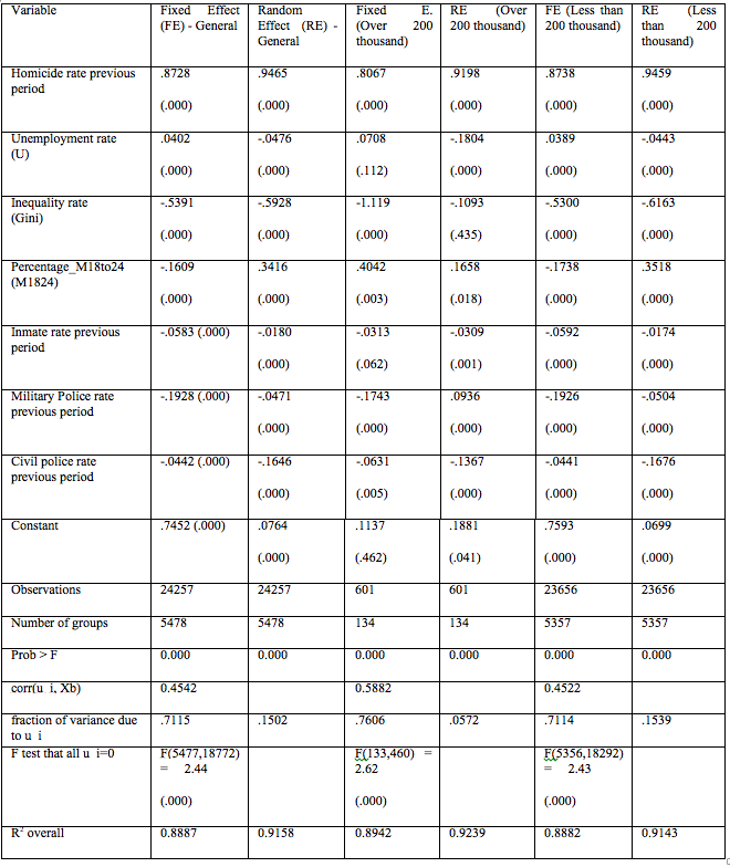
Table 3 repeats the estimates, but this time we adopted a methodology that deals with the specific effects of each place differently, using a data panel model with fixed effects. We point out that, given the characteristics of our sample, the estimate using random effects seem to be more adequate (after all, there are over 5000 cross-section units). Regardless, given the computational ease, we will also show the fixed effect estimates whenever possible.
In regards to the control variables, there are not great qualitative differences between this and the previous result. On the other hand, the results for crime repression variables, although qualitative similar, present more expressive magnitudes. For example, an increase of 1% in the incarceration rate in the previous period can reduce the homicide rate in 0.07%. And an increase in the military police rate can reduce the homicide rate in 0.13%.
Table 3: Determiners of State Homicide rate*. Panel data, fixed effect.
Variable |
General |
Over 1 million inhabitants |
Between 500 thousand e 1 million |
Between 200 thousand e 500 thousand |
Between 50 thousand e 200 thousand |
Less than 50 thousand |
State Homicide rate _previous period |
.9076 (.000) |
.9096 (.000) |
.8252 (.000) |
.7863 (.000) |
.8632 (.000) |
.9137 (.000) |
Unemployment rate (U) |
.0020 (.661) |
-.0863 (.405) |
.0343 (.654) |
.0284 (.413) |
-.0373 (.026) |
.0052 (.274) |
Inequality Rate (Gini) |
-.8114 (.000) |
-.9179 (.041) |
-.7146 (.046) |
-1.091 (.000) |
-.8913 (.000) |
-.8010 (.000) |
Percentage_M18to24 state (M1824) |
-.3516 (.000) |
-.0527 (.800) |
.0942 (.706) |
.3321 (.006) |
.0018 (.973) |
-.3997 (.000) |
Inmate rate previous period |
-.0679 (.000) |
-.0547 (.252) |
-.0130 (.718) |
-.0327 (.053) |
-.0529 (.000) |
-.0701 (.000) |
Military police officer Rate previous period |
-.0597 (.000) |
-.1340 (.018) |
-.0166 (.595) |
-.1195 (.000) |
-.0863 (.000) |
-.0575 (.000) |
Civil Police officer _rate previous period |
-.0149 (.000) |
-.0005 (.977) |
-.0065 (.744) |
-.0142 (.121) |
-.0156 (.000) |
-.0143 (.000) |
Constant |
.4959 (.000) |
.4270 (.079) |
.0087 (.975) |
.0479 (.705) |
.3056 (.000) |
.5267 (.000) |
Observations |
31565 |
90 |
126 |
535 |
2626 |
28188 |
Number of groups |
5478 |
16 |
27 |
101 |
482 |
4930 |
Prob > F |
0.000 |
0.000 |
0.000 |
0.000 |
0.000 |
0.000 |
corr(u_i, Xb) |
0.3669 |
0.1557 |
0.4226 |
0.6792 |
0.6350 |
0.3349 |
fraction of variance due to u_i |
0.6522 |
0.8057 |
0.7257 |
0.7953 |
0.6947 |
0.6520 |
F test that all u_i=0 |
F(5477, 26080) = 4.02 (.000) |
F(15, 67) = 4.06 (.000) |
F(26, 92) = 4.02 (.000) |
F(100, 427) = 4.87 (.000) |
F(481, 2137) = 3.88 (.000) |
F(4929, 23251) = 3.95 (.000) |
R2 overall |
0.8980 |
0.7972 |
0.8949 |
0.9064 |
0.9181 |
0.8954 |
*: all variables in logarithms. t-prob between parenthesis
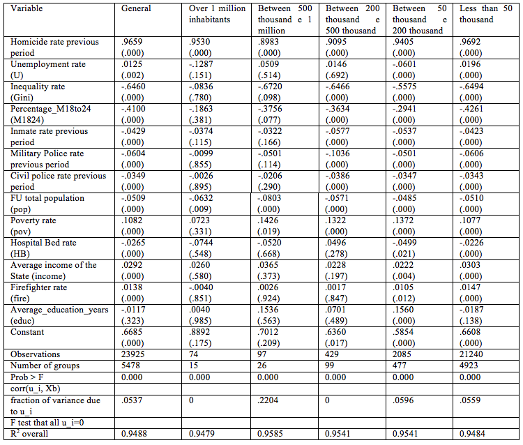
Table 4 includes a new group of control variables to verify the robustness of the results of the crime repression variables. In this table are included the variables regarding the total population, poverty rate, the number of hospital beds, the average income, the number of firefighters, and the average of school years of the population of the state. All these variables are commonly used in studies of violence. The inclusion of those shows that our results, in regards to the crime repression variables, are robust even when new control variables are included.
Table 4: Determiners of State Homicide rate *. Random effect, new proxies
*: all variables in logarithms. t-prob between parenthesis
Table 5 (Annex) repeats the exercise in Table 4, but now using a fixed effect estimator. Again, the inclusion of a new series of control variables did not qualitatively affect the results of the crime repression variables.
Table 6 (Annex) makes the analysis slightly more sophisticated from the econometric point of view. We will now adopt a panel estimative using instrumental variables, such as commonly suggested in the literature. We will use the ratio of military and civil police officers as instruments. The instruments used are those commonly adopted in the national and international literature, and are described in the end of Table 6. Again, all crime repression variables are statistically significant to reduce the homicide rate. However, there is an important quantitative difference: now the elasticity of the ratio of police officers on the homicide rate has a much more expressive magnitude. For example, an increase in 1% in the ratio of military police officers can lower the homicide rate in 0.19%. This effect can be translated as a reduction of 0.13% in the case of civil police officers. The magnitude of the elasticity of the incarceration rate has also increased. An increase in the incarceration rate of 1% can lower the homicide rate in 0.05%.
The central objective of this study was to analyze the effect of crime repression policies in the homicide rate in the society. Crime repression policies can be divided in two groups: incapacitation policies and detention policies. In terms of public policies, the incapacitation is translated as a higher incarceration rate. The detention policy can be understood as an increase in the rate of police officers (both civil and military).
Using a completely new data bank, made up exclusively by official Brazilian government data, we were able to gather information on over 5000 minimum comparable areas from 2003 to 2009. Besides the information regarding the homicide rate and the crime repression variables (incarceration rate and policing rate), we have also gathered data referring to a series of other variables commonly used in studies on criminality. Thus, our study was able to isolate the effects of the repression variables from the social-economic variables (unemployment rate, income concentration, level of education, average income, demographic density, etc.), and also from the demographic effects (rate of young males in the hole population) and the inertia of the homicide rate.
We must highlight that by using a sample made up of MCAs, we were able to introduce a specific component for each place. This is an important innovation in this paper. As far as we know, this is the first time it was done in studies about the homicide rate. Such procedure casts doubts on the possibility of reducing the income inequality as a means to reduce the homicide rate. That is to say, that are certainly beneficial effects in reducing the income concentration, however, homicide rate reduction cannot be counted as one of them.
In general terms, our results regarding the repression variables are robust to a series of different groups of data and alternatives estimations. As a rule of thumb, we have that arresting more criminals and having more police officers on the streets are policies that work in reducing the homicide rate. Thus, this paper aims to demonstrate that great social changes are not necessary to reduce the homicide rate. On the contrary, increasing incarceration rates and police officer rates are public policies capable of reducing the homicide rate, regardless of reducing income inequality, or increasing the average of school years of the population.
We are not arguing against the reduction of income inequality or against the increase in the level of education of the population. We are only pointing out that reducing criminality can be successfully done without major socio-economic changes in society. Putting criminals in jail and increasing the number of police officers are good strategies in reducing the homicide rate. We are not arguing that they are the most efficient strategies, only that they do work.
Baltagi, B. H. (1995). Econometric Analysis of Panel Data, New York: John Wiley & Sons.
BECKER, G. S. (1968). "Crime and Punishment: An Economic Approach". Journal of political economy, v. 76, p. 169-217.
CORMAN, H.; MOCAN, H. N. (2000). "A time-series analysis of burglary, deterrence, and drug abuse in New York city". American economic review, v. 90, n. 3, p. 584-604, June.
Deaton, A. (1985). "Panel data from a time series of cross‐sections", Journal of Econometrics 30 , pp. 109–126.
D'ALESSIO, S. J.; STOLZENBERG, L. (1998). "Crime, arrests, and pretrial jail incarceration: an examination of the deterrence thesis". Criminology, n. 36, p. 735-762.
DONOHUE, J.; LEVITT, S. D. (2001). "The impact of legalized abortion on crime". Quarterly journal of economics, v. 116, n. 2.
DRACA, M.; MACHIN, S.; WITT, R. (2011). "Panic on the streets of London: police, crime and the July 2005 terror attacks". American economic review, 101 (August).
DRAGO, F.; GALBIATI, R. (2010). "Indirect effects of a policy altering criminal behavior: evidence from the Italian prison experiment". Germany: IZA, (Discussion Paper, n. 5.414).
HARCOURT, B. E. (2011). "An institutionalization effect: the impact of mental hospitalization and imprisonment on homicide in the United States, 1934–2001". Journal of legal studies, v. 40, n. 1, Jan.
HSIAO, C. Analysis of panel data. (2003). "Econometric society monographs", Cambridge University Press; 2 edition (March 17)
LOUREIRO, P. R. A.; Mendonça, Mario J. C de; Moreira, Tito B. S. and Sachsida, Adolfo (2009). "Crime, economic conditions, social interactions and family heritage". International review of law and economics, v. 29, n. 3, p. 202-209, Sept..
MACHIN, S.; MEGHIR, C. (2004). "Crime and economic incentives". Journal of human resources, Wisconsin, v. 39, n. 4.
Menezes, Tatiane; Silveira-Neto, Raul; Monteiro, Circe and Ratton, José L. (2013). "Spatial correlation between homicide rates and inequality: evidence from urban neighborhoods". Economics Letters, Vol.120, No.1.
RAPHAEL, S.; WINTER-EBMER, R. (2001). "Identifying the effect of unemployment on crime". Journal of law and economics, v. 44, p. 259-283.
SACHSIDA, A.; LOUREIRO, P. R.; CARNEIRO, F. G. (2005). "Crime and social interactions: a developing country case study". Journal of socio-economics, v. 34, n. 3, p. 311-318.
SACHSIDA, A.; LOUREIRO, P. R.; MENDONCA, M. J. C. (2002). "Interação social e crimes violentos: uma análise empírica a partir dos dados do presídio de papuda". Estudos econômicos, v. 32, n. 4, p. 621-642.
SACHSIDA, A.; MENDONCA, M. J. C. (2007). "Ex-convicts face multiple labor market punishments: estimates of peer-group and stigma effects using equations of returns to schooling". Revista ANPEC, v. 8, p. 503-520.
SACHSIDA, A.; Mendonça, Mario J. C. de; Loureiro, Paulo R. A.; Gutierrez, Maria B. S. (2010). "Inequality and criminality revisited: further evidence from Brazil". Empirical economics. v. 39, n. 1,·p. 93-109.
Table 5 - Determiners of State Homicide rate *. Fixed effect, new proxies
Variable |
General |
Over 1 million inhabitants |
Between 500 thousand e 1 million |
Between 200 thousand e 500 thousand |
Between 50 thousand e 200 thousand |
Less than 50 thousand |
Homicide rate previous period |
.6902 |
.7097 |
.5877 |
.5630 |
.6454 |
.6969 |
Unemployment rate |
-.0034 |
.0085 |
.0211 |
.0917 |
-.0031 |
-.0069 |
Inequality rate |
.2887 |
.6405 |
.5255 |
.2268 |
.6328 |
.2479 |
Percentage_M18to24 |
.4260 |
.4932 |
1.334 |
.9731 |
.6121 |
.3868 |
Inmate rate previous period |
-.0633 |
-.0432 |
.0217 |
-.0361 |
-.0452 |
-.0662 |
Military Police rate previous period |
-.0501 |
-.1136 |
-.0196 |
-.1080 |
-.0749 |
-.0460 |
Civil police rate previous period |
-.0044 |
.0009 |
.0095 |
-.0043 |
-.0138 |
-.0031 |
FU total population |
-.8027 |
-.3041 |
-1.189 |
-1.409 |
-1.441 |
-.7280 |
Poverty rate |
-.0581 |
-.2363 |
-.0830 |
-.0832 |
-.0994 |
-.0511 |
Hospital Bed rate |
.1485 |
-.0467 |
1.104 |
.0140 |
.2097 |
.1443 |
Average income of the State (income) |
-.0389 |
-.1030 |
-.0199 |
-.0718 |
-.0491 |
-.0367 |
Firefighter rate |
.0065 |
-.0165 |
-.0444 |
-.0064 |
.0013 |
.0078 |
Average_education_years |
1.631 |
1.203 |
2.402 |
2.109 |
1.813 |
1.603 |
Constant |
4.532 |
2.396 |
3.633 |
8.717 |
8.944 |
4.027 |
Observations |
23925 |
74 |
97 |
429 |
2085 |
21240 |
Number of groups |
5478 |
15 |
26 |
99 |
477 |
4923 |
Prob > F |
0.000 |
0.000 |
0.000 |
0.000 |
0.000 |
0.000 |
corr(u_i, Xb) |
-0.8642 |
-0.5096 |
-0.9502 |
-0.9611 |
-0.9497 |
-0.8377 |
fraction of variance due to u_i |
.9898 |
.9368 |
.9958 |
.9977 |
.9963 |
.9877 |
F test that all u_i=0 |
F(5477, 18434) = 3.15 |
F(14, 46) = 2.17 |
F(25, 58) = 3.51 |
F(98, 317) = 4.04 |
F(476, 1595) = 3.08 |
F(4922, 16304) = 3.13 |
R2 overall |
0.2074 |
0.4907 |
0.3820 |
0.2535 |
0.2142 |
0.2157 |
*: all variables in logarithms. t-prob between parenthesis
Table 6: Determiners of State Homicide rate *. Instrumental variables panel.
*: all variables in logarithms. t-prob between parenthesis. Instrumental variables: Military police officer Rate previous period and Civil Police officer rate previous period. Instruments used: all variables included in the equation (added the first lag) of the following variables – Total Population by State , Poverty rate, Hospital bed rate, Average income of the state, Firefighter rate, Average_education_years.
1. Pesquisador do IPEA. Técnico de Planejamento e Pesquisa da DIRUR. E-mail: sachsida@hotmail.com
2. Pesquisador do IPEA. Técnico de Planejamento e Pesquisa da DIMAC. E-mail: mario.mendonca@ipea.gov.br
3. Professor e pesquisador do Departamento de Economia da Universidade Católica de Brasília. E-mail: tito@pos.ucb.br
4. Professor e pesquisador do Departamento de Economia da Universidade de Brasília: E-mail: puloloureiro@unb.br
5 These are in fact cities transformed into minimum comparable areas.
6. Some papers about criminality in Brazil can be highlighted, among those are: Sachsida et. all (2002); Sachsida, Loureiro and Carneiro (2005); Sachsida and Mendonça (2007); Loureiro, P. R. A. et. al. (2009), Sachsida et. al. (2010) and Menezes, T. et. al. (2013).
7. In fact, cities in the whole country were used. New cities were created and there were some changes in the cities in the base year 1997 through time. We were careful to take such changes in consideration and transform the cities into minimum comparable areas.
8. More details on the panel data estimator can be found in Baltagi (1995), Hsiao (2003) or Deaton (1985).