ISSN 0798 1015

Vol. 39 (Number 19) Year 2018 • Page 31

Innovative system of estimation of investment projects of development of subjects of regional economic complexes on the basis of combined methods of computer optimization

Sistema innovador de estimación de proyectos de inversión de desarrollo de sujetos de complejos económicos regionales sobre la base de métodos combinados de optimización informática

Bulat A. AKHMADEEV 1; Sergey V. MANAKHOV 2

Received: 05/03/2018 • Approved: 25/03/2018

Content

1. Introduction

2. A numerical model for optimization calculations

3. The solution of the dual problem

4. Updating constraints to solve the problem for the next period

5. Solution of the prediction task for several periods

6. Conclusions and future work

References

1. Introduction

There comes the time of the project economy - projects should be properly evaluated, it is necessary to set the right priorities for successful economic planning. Planning is not advisable on a super-detailed level (for example, to plan how many ice cream units should be produced), since the economy has a self-regulating property. However, at the level of major economic projects, it is sometimes a necessary regulation by the state. Management and optimization of project activities by the state can positively affect the "healthy" functioning of other sectors of the economy associated with a particular project by various financial and commodity relations.

First of all, optimal planning deals with monetary investments in the most critical parts of the system (or industry), because finance is the circulatory system of any economy. Proactive adjustment by the state in the timely regulation of the economy is relevant especially in the situation of external geopolitical instability associated with import and export risks, as well as in identifying critical shortages of any resources (commodity, human or financial) in the economy (Demenko et al., 2017). This requires an adequate system for diagnosing the economic situation and timely competent regulation and planning. Therefore, the question arises of choosing a diagnostic mechanism, i.e. economic models and tools.

It is known that the existing macroeconomic models of the general dynamic stochastic equilibrium are fragmentary and largely contradictory, and also overwhelmed by a significant number of theoretical assumptions, parameters and conventions that are impossible or very difficult to estimate in the real economy (see, for example, the Ramsey (1929), Arrow and Debreu 1954), Samuelson (1956), Tobin (1969), Shapiro and Stiglitz (1984), Blanchard and Fischer (1989), Bernanke, Getler (1995), etc.), which prevents them from being used directly for application analysis and planning.

In turn, econometric models based on the analysis of statistical data and the identification of interrelations between economic processes do not require the imposition of a large number of a priori assumptions about the system under investigation and rely almost entirely on empirical data (e.g. Moiseev, 2017). However, a significant drawback of models of this type is the possible classification of false found relationships as true. Since in the economy at the macro level it is difficult to conduct experimental experiments, then with the help of econometric methods it is quite difficult to identify valid true interrelations, on the basis of which it is possible to make competent managerial decisions.

Later agent-based models (ABM) of the economy in many respects surpass in their capabilities and practical applications the abovementioned ones. A distinctive feature of these models is the so-called "bottom-up" modeling or decentralized modeling, when the general behavior of the system is not known initially, and only the individual characteristics and algorithms of agent behavior are known (Makarov and Bakhtizin (2013)); The areas of application of ABM in the economy are quite broad: starting from the financial sphere (see, for example, Raberto et al. (2001), LeBaron (2006), Moiseev and Akhmadeev (2017)), Production (Kutschinski et al. (2003)), labor market (Tassier and Menczer (2001)), innovation (Dawid (2006), Akhmadeev and Manakhov (2015)), business cycles (Delli Gatti et al. (2008) and many others). The advantage of ABM in comparison with the classical economic models of general equilibrium lies in the maximum approximation of the structure of models to real socio-economic processes and phenomena. However, the success of the application of these models depends largely on the skill of their development and adaptation. Advantages can turn into disadvantages in the unprofessional construction of excessively detailed and loaded with a large number of parameters models, not applicable in practice.

Another class is the models of optimal planning (OP), based on the tools of mathematical programming. This type of models was widely used in the middle of the last century not only in the planned economy of the USSR, but also in capitalist countries, for example, in the USA (see the well-known model of the inter-branch balance of Leontiev (1951)). In Russia, the founder of the idea of ​​optimal planning was Academician L.V. Kantorovich (Kantorovich, 1959). In the USSR, this type of model was intended for a planned economy (Kantorovich et al., 1970), but under the conditions of transition to a market economy, the tasks of the OP themselves change significantly - it should be widely applied within individual companies (enterprises), but on a nationwide scale, it can acquire not a directive and detailed but a more indicative and extended character.

The principle of optimal planning in combination with the method of economic analysis based on cross-industry input-output tables is a perfect visual instrument for analyzing the state of the economy. In this study, an attempt is made to combine the methods of ABM and linear programming to construct the most appropriate project planning and evaluation system for the Russian economy.

The aim of the work is to develop a planning tool for optimization of economic projects, including a study of the impact of interest rates on loans, tax rates, the level of accumulation in fixed assets, as well as other control parameters based on the combined method of mathematical and computer programming. On a very simplified numerical example, it is shown that the effectiveness of the project depends on different factors. The most significant factor is the criterion for evaluating the project. There are many criteria, we list some. The most popular among economists of the old school is the payback period of the monetary costs invested in the project. But even in the use of this criterion there may be nuances. The profit can be returned to the investor, public or private. It can go to different project executors or it can change the distribution of ownership, etc. A fundamentally different criterion is the execution of the project as soon as possible. Another criterion is the best satisfaction of the workers performing the project. In general, the time factor in project evaluation plays a critical role. In our conditional example, we show how the effectiveness assessment changes if in one time interval the project goal and, therefore, the criterion, is one, and in the other, it is substantially adjusted.

Further, we specially pay attention to the difference in the nature of the "products" appearing in the optimization model. The word "product" is specially taken in quotation marks. The product can be money, inventions, intangible masterpieces of art, etc.

On a simple numerical example, we specifically refer to such a product as money. Money as costs are represented in all modes of production. And to produce them, i.e. "to print", for the government literally costs nothing. Therefore, the problem arises of the optimal amount of money. The task is complex, affecting all aspects of the economy. Much more difficult than the formulas known from the textbooks for the connection of the quantity of money, GDP and inflation.

The main question, illustrated by the calculations in the given example, is how to evaluate the effectiveness of a new project depending on a number of factors, including the criteria for optimality, lending rates, etc.

2. A numerical model for optimization calculations

Hereafter, the paper considers a simplified formal representation of projects as vectors whose components show the receipt of goods (products, money) if the number is positive, and the costs measured by negative numbers. Opportunities of the economy as a whole are also described by a set of vectors showing the possibilities for production, financing, employee behavior, investments in fixed assets, etc.

The original description of the economy follows the classic work of Kantorovich (see Kantorovich, L.V. (1959)). The essential difference is only that the products are, in particular, money.

The algorithm of calculations, with the help of which the optimal solution is determined by a given criterion, is a sequence of actions, among which the main is the solution of the optimization problem, later called the reference problem.

The following numerical calculations contain two directions. The first is the optimal trajectory of the economy, depending on several accepted in practice criteria. The second assesses the effectiveness of new projects for implementation in practice, also depending on the initial data and the criteria for optimality.

The model is a closed-type financial system where various types of economic agents are present: banks lending to producers of goods, as well as the population for the realization of final consumption, the producers of various types of products that make profit in the form of surplus value, the population that carries out final consumption, which spends the salary, and in case of its shortage, takes a loan from the bank, investment and other projects, as well as the state that is carrying out project financing perspective projects, which also presents in the model of the researcher-optimizer, who himself exposes the necessary criterion of optimality of the solution of the problem.

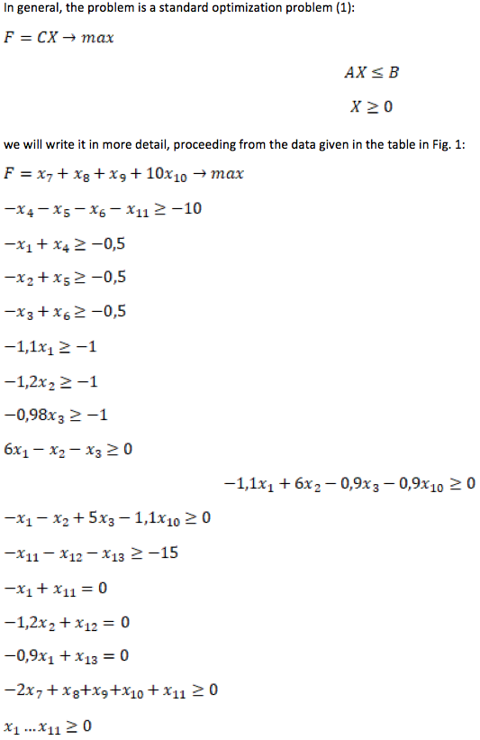
We describe the problem in more detail, for this we define the optimization problem (local - for the 1st year) below:

There are many N "production methods" or agents where the intensity of the j-th method is expressed in terms of xj and determines the level of execution of this method (for example, the production of a particular product). Below is a simplified numerical example of the optimal planning problem:

1) 3 agents, each of which produces its type of goods, they can express 3 separate enterprises.

2) 3 agents engaged in lending to each of the above production methods,

3) 1 agent, carrying out the realization of final consumption (population),

4) 1 an agent that lends to the population,

5) 3 agents expressing the movement of labor from one producer to another.

Each agent has its own production parameters or "resources", where the sign in front of the parameter values determines whether it is cost or output. In this task, we have 15 different products: 1) a central budget that simultaneously performs the function of a central bank, 2) the financial costs of three manufacturing enterprises, 3) the use of fixed assets of three manufacturing enterprises, 4) the production matrix or costs and output products by three production enterprises, 5) available resources of labor, 6) labor requirements of three production enterprises, 7) expenditures of the population for final consumption (own financial resources or credit funds).

The graphical representation of this table is shown in Fig. 1:

Figure 1
Optimization tasks for the 1st year.

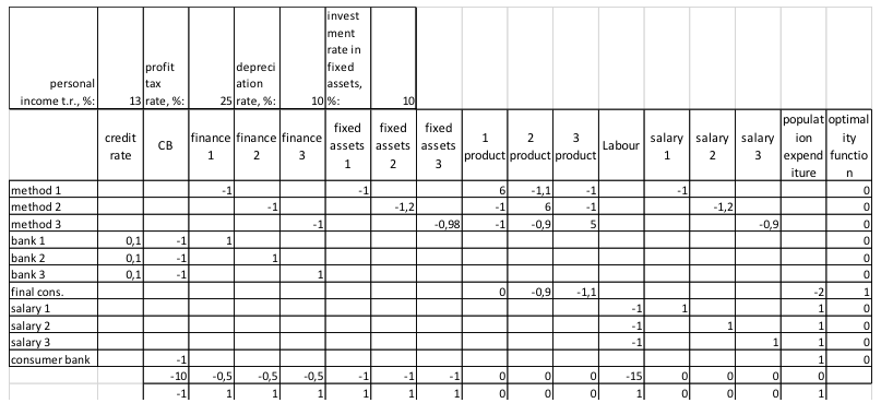
We describe in detail the proposed production methods with their parameters, constraints and the criterion of optimality.

The table consists of a production matrix A, consisting of n rows or "production methods" (agents) and m columns or "resources" (parameters). The last column in Fig. 1 is the vector of the optimality criterion C that is not in the matrix A. The second line from the bottom - vector B - restrictions on resources: financial costs, production assets, labor, etc. The last line expresses the restriction on the resource bj in the vector B: 1 means ">", 0 means "=" and -1 means "<". This line is needed to solve the optimization problem in the Wolfram Mathematica computing environment.

The solution of the reference problem to a maximum

The optimization task is to maximize the final consumption of products with a coefficient of 1 (see Fig. 1).

The Wolfram Mathematica programming environment automatically brings the constraint system to the canonical form.

After solving this problem, the program finds the values ​​of the vector X, i.e. intensity of performance of each of the production methods. Table 1 shows the results of solving a direct problem for the first period:

Table 1. The result of solving the problem for the first period.

Let's make a brief analysis: as it is clear from the solution of this problem, the production enterprise No. 1 did not use the loan issued by the central bank (x4=0.00), and the intensity of the manufacturing mode of the enterprise No. 1 (x1) is 0.30, which could occur due to a deficit of one of the resources , which will be discussed below when solving the dual problem. And the enterprise 3 has worked above the norm of its power, the intensity of the production method (x3) is equal to 1.02. As was said above, in this problem the only criterion of optimality is the maximization of final consumption. The intensities of production methods are set by the solution of the optimization task in such a way as to give the maximum final consumption within the limits of the available resource constraints.

This problem of linear programming is described by L.V. Kantorovich in his famous book (Kantorovich 1959), for which he received the Nobel Prize. The difference between the present model is that not only ordinary institutions, funds and services appear as products (parameters), but also money itself. This is discussed in more detail below.

In order to analyze the results of solving this optimization problem, it is necessary to solve the dual problem, as well as to perform the necessary calculations to construct the problem for the next period.

3. The solution of the dual problem

The solution of the dual problem involves finding the so-called objectively-based estimates (shadow prices) on each of the resources. In the classical optimization problem, the solution of the dual problem means finding shadow prices for the resources indicated in the constraints (vector B), at the sale of which we would receive an income no less than that generated in the case of using resources for production in our ways, with the revenue or price on sale of the output indicated in the vector C. In the classical form it is formulated as follows:

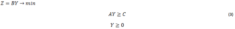
Where B is the resource vector, A is the production matrix, and Y is the shadow prices.

The Wolfram Mathematica system solves this problem automatically from the source data, so you do not need to transpose the constraint matrices and prepare the data to solve it. In Table 2 the resource estimates (shadow prices) for resources are shown for solving the dual problem for the 1st period:

Table 2. The result of the solution of the dual problem for the first period.

Further, knowing the shadow prices for product 1 (y8=0.16), product 2 (y9=0.16), and product 3 (y10=0.78), we can determine the scarcity of each resource. The mathematical meaning of these estimates lies in the fact that they determine how much the value of the objective function will increase (decrease) with increasing (decreasing) the stock of the given resource by one unit. In our case, the most scarce product is No. 3 with the estimate equal to 0.78, and also there is a high shortage of fixed assets for the same enterprise №3 (y7) with an estimate equal to 3.68, from which we conclude that having increased the volume of fixed assets for enterprise №3 and, accordingly, having produced more product number 3, we will achieve a larger increase in the objective function, because as it was proved above in solving the main problem, an increase in the intensity of the production process (production of product No. 3) gives a greater increase in the final consumption (objective function).

4. Updating constraints to solve the problem for the next period

Let's write down the step-by-step algorithm of data recalculation for solving the prognostic problem for several periods:

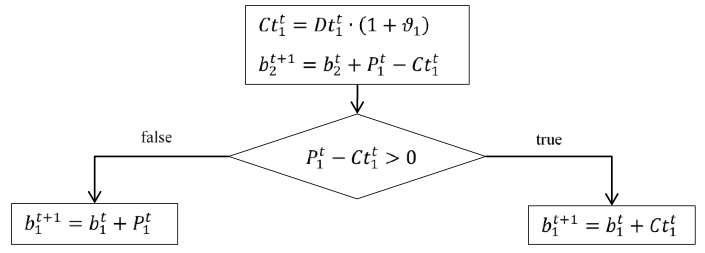
1) Let's show how the profit for the enterprise №1 is considered: the intensity of the production method is determined through x1, by this value we multiply the amount of operating costs, the difference between direct costs and income from sales of manufactured products, labor costs and depreciation on the fixed prices, also deducting an income tax:

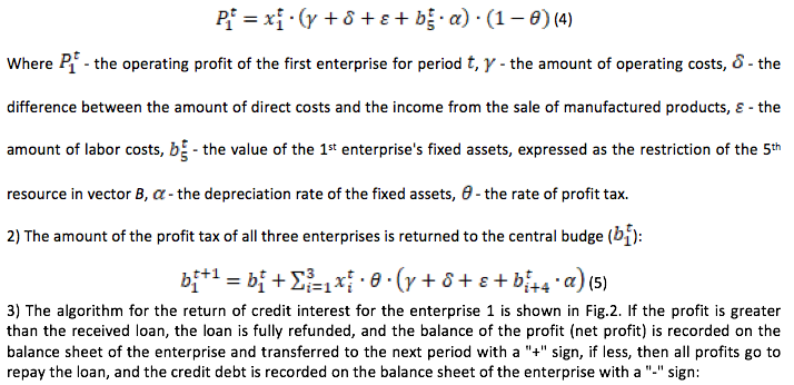
Figure 2
Algorithm for the return of credit money to the budget

5. Solution of the prediction task for several periods

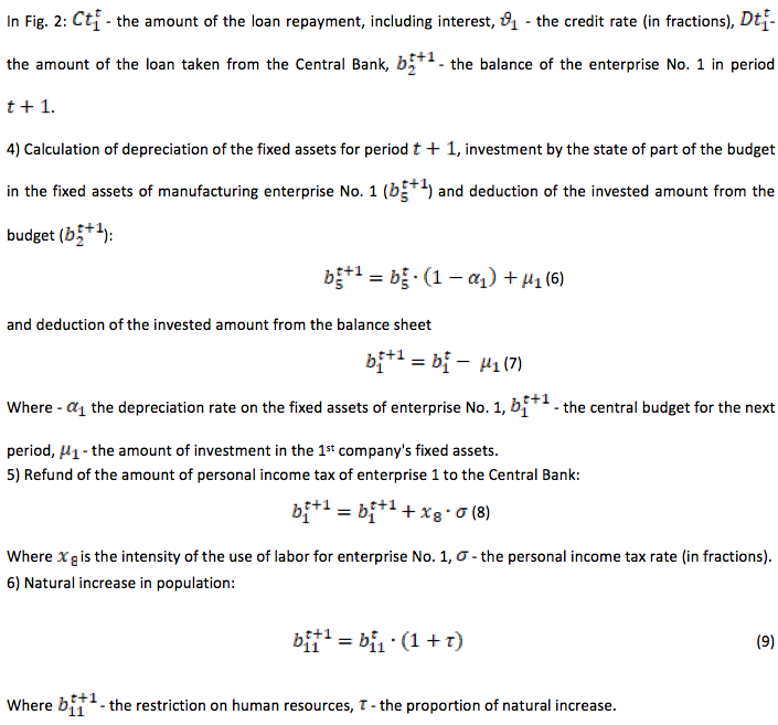
After determining the main parameters of the problem and the formulas for calculating them for the next period, the problem of algorithmic prediction for several periods is solved. The essence of the algorithm is to use the economic meaning of the shadow prices for adjusting the size of investments in the fixed assets with the aim of increasing the volume of final consumption in the long term. That is, invest more money in the fixed prices of more scarce products. The amount of investment, according to formula (6) is determined by a fixed rate and is appointed exogenously by the central apparatus (state).

The algorithm described below assumes that the state, based on the decision of the overall optimization task, invests the adjusted amount in the projects. For example, if the level of deficiency of product No. 1 in the previous period was 0.78, then this amount is invested in the fixed assets of the enterprise producing product No. 1.

Accordingly, in the formula (6) the parameter is corrected as follows:

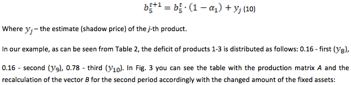
Figure 3
Limitations of parameters with recalculation for the 2nd period.

When solving the prediction task for several periods, this operation is performed at the end of each period. Next, we will carry out a series of experiments.

Experiment 1 - investment based on objectively-based estimates (shadow prices)

Next, we will conduct the following experiment in two modes:

1) we invest in the fixed assets of the three enterprises not a fixed rate, but the amount expressed in the scarcity estimate of this resource (shadow price);

2) we invest a fixed amount equal to the average amount of investments in the 1st mode, so that the total amount of investments is the same.

We solve the optimization problem with a calculation for 50 periods. As indicators of effectiveness we will take: 1) the level of final consumption, 2) the volume of the central budget; 3) the financial balance of the three enterprises (the total amount) it the 50th period in both cases; 4) the ROI (return on invested capital), which is the ratio of total income to total investment for all simulation periods.

Table 3
Experiment to assess the effectiveness of investment in fixed assets

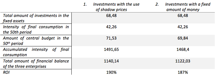
The results of the experiment in Table. 3 show that for all indicators, except the level of final consumption in the 50 period, the 1st experiment mode shows better results and, accordingly, more efficient allocation of investment funds in the economy.

Figure 4
ROI value for accumulated investments and accumulated return for 20 modeling periods.

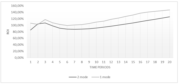
The graph in Fig. 4 shows that the experiment in 1 mode shows the return on investment (ROI) - an average of 20% higher.

Experiment 2 - search for parameters that maximize the utility function.

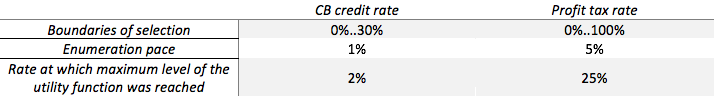
This experiment is carried out by numerical selection of optimal control parameters, which were chosen as the rate of profit tax and the credit rate of the central bank. As a utility function, the accumulated central budget indicator was selected for 50 modeling periods (see Table 4):

Table 4
Initial data and experimental results

In Fig. 5, the values of the control parameters along the x (credit rate) and y (profit tax rate) axes, as well as the values of the objective function along the z (central budget) axis, are visually demonstrated.

Figure 5
Three-dimensional representation of the results of the experiment with
the utility criterion (axis z) - the level of the accumulated budget

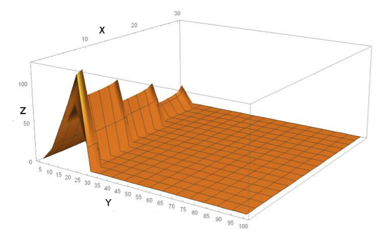
Thus, as a result of experiment No. 2, the optimal rates for loans and income tax were identified. When compared with real rates in the Russian Federation, the profit tax is almost at the same level (24% in the Russian Federation), but the loan rate in the Russian Federation (on average 10%) is much higher than the optimal rate, according to the experiment conducted above.

Figure 6
Three-dimensional representation of the results of the experiment with the
criterion of utility (axes z) - the level of final consumption and the same control
parameters along the axes x and y.

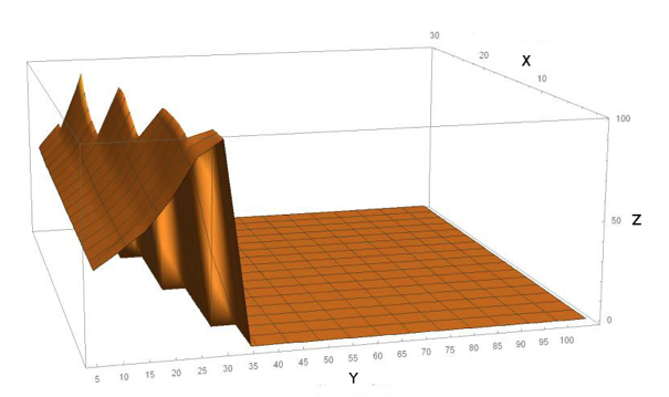
Fig. 6 clearly shows that the level of final consumption does not depend on the change of these parameters, however, there are permissible limits within which the population of manufacturing companies continues to exist while remaining profitable. For example, with a profit tax rate of more than 40%, one or more companies do not survive to 50 modeling periods, becoming unprofitable. Comparing these two optimality criteria (Figures 6 and 7), we can conclude that the regions of admissible values ​​in both cases roughly coincide.

Experiment 3 - evaluation of the effectiveness of commissioning a new project.

Above we demonstrated the possibilities of the system on the simplest numerical examples with 3 enterprises producing products No. 1, 2 and 3, each with its own efficiency and the amount of resources used. For this experiment, a new example was chosen with 4 enterprises and new values ​​of production matrix A.

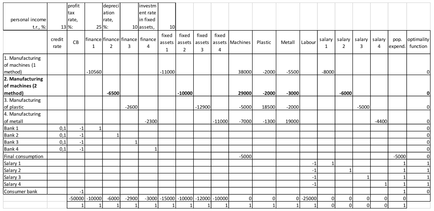
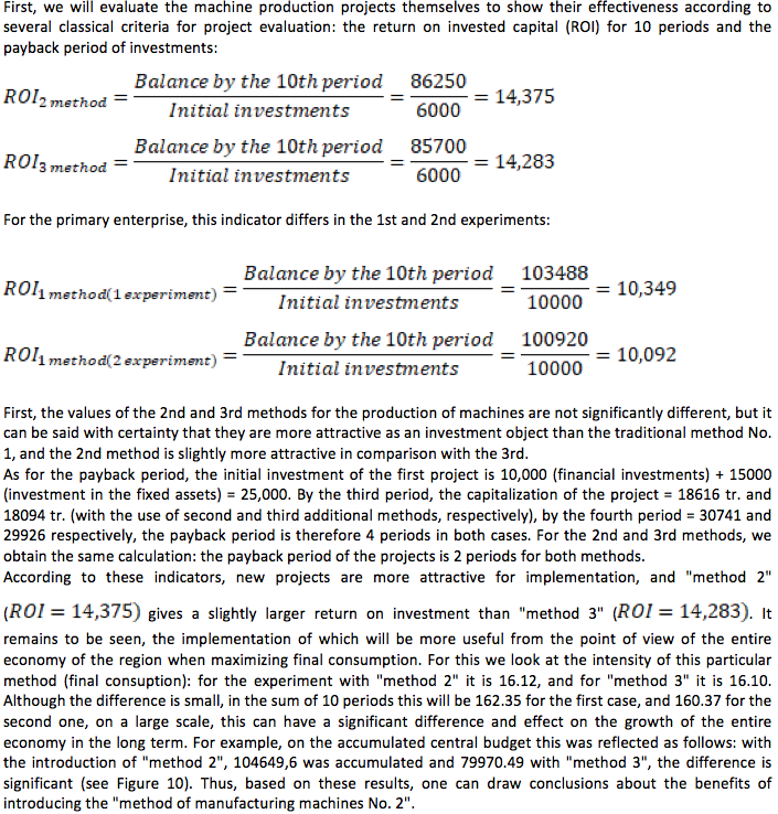
Suppose that the machine-building industry is developed in a certain region, and the region's leadership decided to modernize this industry with new production methods (innovations) and announced a competition for projects on the production of machines, to which two completely new enterprises that had not worked in the region had submitted their business projects. For the convenience of analysis, the economy model is simplified to produce 3 different products: "machines", "metal" and "plastic." The traditional method of production is called "method 1", and two new methods are "method 2" (see Figure 7) and "method 3" (see Figure 8). Now the product "machine" can be produced not only by basic, but also by an additional original method, which will have a different production efficiency. Next, experiments will be performed with a comparison of the effectiveness of these additional (different from each other) methods of manufacturing machines under various optimality criteria. Thus, we show how projects can be evaluated not only from the point of view of the profitability of enterprises and the classically accepted financial indicators of project evaluation (ROI, the payback period of investments, etc.), but also from the standpoint of the effectiveness of a particular project for the entire economy, what we will consider good: the increase in the central budget, the increase in final consumption, the profits of the companies themselves, or the growth of wages for the population, etc.

Figure 7
Commissioning of a new project for the production of machines (2nd method).

-----

Figure 8
Commissioning of a new project for the production of machines (3nd method)

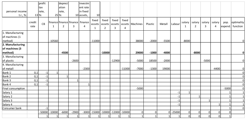
As you can see in Fig. 7 and 8, the method of producing machines 2 and 3 is characterized by the consumption of a number of different resources, for example, method 3 consumes more metal (4000), but less plastic (1000) compared to method 2 (3000 and 2000, respectively), the initial financial investment and the fixed assets are allocated to both projects in the same amount. Profit tax (25%), personal income tax (13%) and depreciation rate (1%) remain at the same level, just as the algorithm for investing in the fixed prices determined in the first experiment.
Let us define the profitability of these projects. We remember that the profit is calculated according to the formula (4). As for the 2nd and for the 3rd method of production of machines, it is equal to 11400 for one period when the intensity of the method is equal to 1, which puts our investment projects in equal initial conditions.
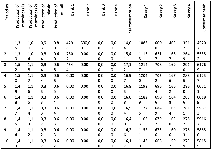
So, let's start the experiments themselves. To begin with, we will select a criterion of optimality standard for the market economy (from the point of view of the region's leadership) - the maximization of final consumption, respectively, we see 1 in the vector C in the line "final consumption" (Figures 7 and 8). In Tables 5 and 6, solutions of the above optimization problems with the intensity of application of each method for 10 simulation periods are given:

Table 5
The intensity of production methods with the addition of
method No. 2 with the maximization of final consumption

-----

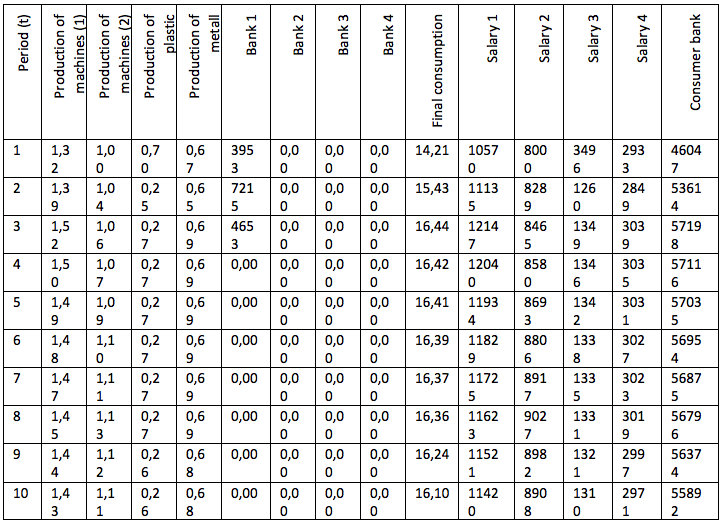
Table 6
The intensity of production methods with the addition of method No. 3 with the maximization of final consumption.

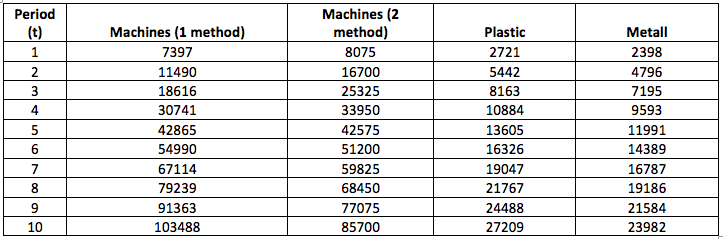
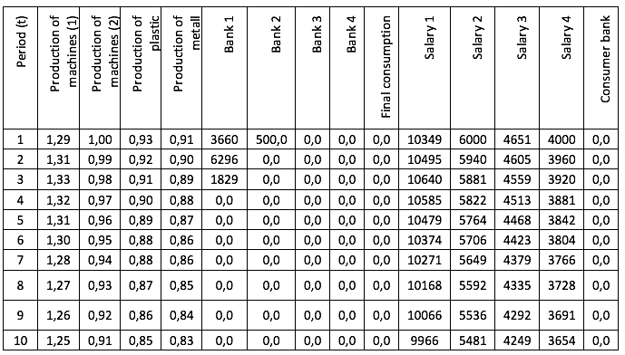
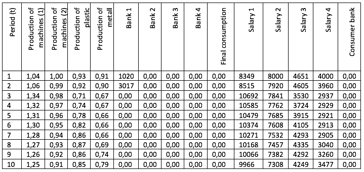
Tables 7 and 8 show the changes in the values of the capital of 4 model enterprises during 10 modeling periods, which we will need for further evaluation and analysis:

Table 7
Change in the capital of 4 enterprises with the introduction of the 2nd method of manufacturing machines

-----

Table 8
Change in the capital of 4 enterprises with the introduction of the 3rd method of manufacturing machines

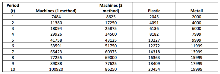
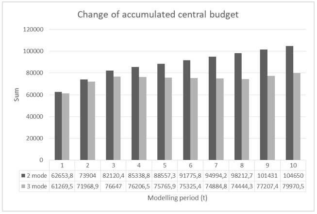
Fig. 9 shows the values of the accumulated central budget for all 10 periods:

Figure 9
Accumulated central budget for 10 periods.

But now let's imagine that the government of the region cares not only about the growth of the economy and about the increasing output of machines, but also about the welfare of the people, and therefore wants to maximize the payment to specialists working in all sectors. Accordingly, we change the values of vector C: for final consumption, we set the value 0, and for wages in all 4 ways we set the value 1. The results of the task of maximizing wages are presented in Tables 9 and 10:

Table 9
The intensity of production methods with the addition of method 2 with the maximization of wages.

------

Table 10
The intensity of production methods with the addition of method 3 with the maximization of wages.

We see that both "method 2" and "method 3" are performed with the same intensity in all periods, but we, as interested in increasing the welfare of the population, are interested in how much it has increased. To do this, let us compare the total intensity of the implementation of the methods for paying wages of all 4 enterprises for 10 periods. According to the first experiment, we get 243485, for the second one - 250000, accordingly, the introduction of "method 3" gives a greater effect on the growth of wages.

Thus, we saw how, depending on the chosen criterion of optimality, various economic projects can be more or less useful for the economy. As in our example, the project for the production of machines No. 2 was more effective for implementation, if our goal was to increase the final consumption and the accumulated budget. On the other hand, if the goal is wage growth, then project number 3 gives the best results. Here we have considered only certain variants of the application of the optimality criterion, although there may be many. For example, if the leadership of the region were interested in increasing the profit of an individual enterprise, then the criterion would be appropriate, and the result would be completely different.

6. Conclusions and future work

The method of computer evaluation of the effectiveness of projects described in this paper can be used in the work of the above-mentioned networks of situational centers. The options for interaction between such situational centers, the leadership of the region and the enterprises working in it can be different.

For example, the management of the enterprise offers a project of modernization of its enterprise and asks the regional authorities to help with financing. The proposed method allows for a full breakdown of options depending on the criteria of optimality, credit rates, price and consumer policies. To carry out the calculations, the situation center should receive information about the enterprise, proposed modernization projects, as well as the financial situation in the country and the region.

We draw the attention of the reader to the fact that the conditional numerical examples given in this paper were used to demonstrate the capabilities of this system. Also, we want to note that the developed system and the capabilities of the Wolfram Mathematica software environment allow to make calculations with any dimension of the matrices. The quantity of both products (parameters) and the projects themselves can be significantly expanded depending on the goals set.

The application of this system for the calculation and evaluation of economic projects based on examples with real projects using tables of interbranch balance is planned in the future works of the authors.

References

Akhmadeev, B. and Manakhov, S. (2015). Effective and sustainable cooperation between start-ups, venture investors, and corporations. Journal of Security and Sustainability Issues, 5(2), 269–285.

Arrow K. and Debreu G. (1954) Existence of Equilibrium for a Competitive Economy. Econometrica, 25, 265-290.

Bernanke B. and Gertler M. (1995) Inside the black box: the credit channel of monetary policy transmission. Journal of Economic Perspectives, 9 (4), 27-48.

Blanchard O.J. and Fischer S. (1989) Lectures on Macroeconomics. MIT Press: Cambridge.

Dawid H. (2006) Agent-based models of innovation and technological change. Handbook Computational Economics 2, 1235-1272

Delli Gatti D., Guilmi C., Gaffeo E., Giulioni G., Gallegati M. and Palestrini A. (2005) A new approach to business fluctuations: heterogeneous interacting agents, scaling laws and financial fragility. Journal of Economic Behavior Organization 56 (4), 489-512

Demenko, O. G., Makarova, I. G. and Konysheva, M. V. (2017). The Origin and Development of Municipal Self-government in Russia   Serials Publications Man In India, 97(20), 381-390

Kantorovich, L.V. (1959). Economic calculation of the best use of resources. Moscow: Publishing House of the USSR Academy of Sciences, pp. 344.

Kantorovich, L.V., Bogachev V.N. and Makarov V.L. (1970). About an estimation of efficiency of capital expenses. Economics and Mathematical methods, 6(6), 811-826.

Kutschinski E., Uthmann T. and Polani D. (2003) Learning competitive pricing strategies by multi-agent reinforcement learning. Journal of Economic Dynamics Control 27, 2207-2218

LeBaron B. (2006) Agent-based financial markets: matching stylized facts with style. In: Colander D. (ed) Post Walrasian macroeconomics op. cit., pp 221-235

Makarov V.L. and Bakhtizin A.R. (2013). Social modeling - a new computer breakthrough (agent-oriented models). Moscow: Economics, pp. 295

Moiseev N. A. (2017). Forecasting time series of economic processes by model averaging across data frames of various lengths. Journal of Statistical Computation and Simulation, 87 (17), 3111-3131.

Moiseev N.A. and Akhmadeev B.A. (2017). Agent-based simulation of wealth, capital and asset distribution on stock markets. Journal of Interdisciplinary Economics, 29 (2), 176-196.

Raberto M., Cincotti S., Focardi S. and Marchesi M. (2001) Agent-based simulation of a financial market. Quantitative Finance Papers

Samuelson P. (1959). An exact consumption-loan model of interest with or without the social contrivance of money. J. of Political Economy, 66(6), 467-482.

Shapiro C and Stiglitz J. (1984) Equilibrium unemployment as a discipline device. American Economic Review, 74 (3), 433-444.

Tassier T and Menczer F. (2001) Emerging small-world referral networks in the evolutionary labor markets. IEEE Transactions, Evolutionary Computution 5 (5), 482-292.

Tobin J. (1969) A General Equilibrium Approach to Monetary Theory. J. of Money, Credit, and Banking, 1.

1. Plekhanov Russian University of Economics, 117997, Russia, Moscow, Stremyanny Ln., 36, E-mail: Bulat.a@mail.ru

2. Plekhanov Russian University of Economics, 117997, Russia, Moscow, Stremyanny Ln., 36, E-mail: sman2003@mail.ru