![]() ISSN 0798 1015
ISSN 0798 1015

![]() ISSN 0798 1015
ISSN 0798 1015
Vol. 39 (Number 33) Year 2018 • Page 32
Diego H. SEGURA 1; Carlos VALENCIA 2
Received: 05/03/2018 • Approved: 12/04/2018
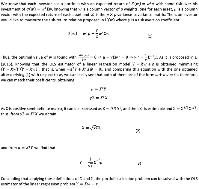
ABSTRACT: The portfolio selection problem can be viewed as a maximization of the risk-return relation based on the input parameters, expected returns and covariance between assets. As these parameters depend on historical market data with stochastic behavior, their real values are not achievable. The estimators haul error that result in under-performance of the selected portfolio. As a solution, we present and analyze a penalized linear regression methodology, which constrains the decision variables to limit the estimation risk of the parameters. |
RESUMEN: El problema de selección de portafolio puede ser entendido como la maximización de la relación riesgo-retorno basada en los parámetros de entrada, retornos esperados y covarianzas entre activos. Estos parámetros dependen de datos históricos del mercado con componente aleatorio y sus valores reales no son conocidos. Los estimadores tienen errores que conllevan a un comportamiento sub-óptimo del portafolio. Como una solución, presentamos y analizamos una metodología de regresión penalizada, restringiendo las variables de decisión para limitar el riesgo de estimación. |

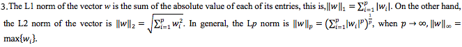
The art of making money in the stock market is indeed an art, as it seems impossible to follow a simple recipe. Investors are differentiated based on their risk aversion profile and their portfolios performances. As the risk aversion profile is intrinsic to the investor, it is possible to study how to choose a better portfolio selection strategy for a given risk. These studies can be agglomerated in what is called “Modern portfolio selection problem”, which has been studied since Harry Markowitz published his paper “Portfolio selection” in 1952 (Markowitz, 1952). In his seminal paper, it is proposed that the investor can select a group of assets of the stock market, wisely choosing a weight that is held in each asset, not only motivated by risk minimization or return maximization, but thinking in the diversification of his investment. Following these ideas, it is possible to think that Markowitz finally created a recipe, an optimization problem that can be easily solved, yet, there is art behind. Although Markowitz created a new framework, it remains conceptual because, as he recognizes, his model does not take into account the uncertainty of its parameters: expected returns of the assets and covariance between them. As we like to maximize the return-risk relation, these model parameters are significantly important. Pitifully, their real values are not easily estimable and then, we can only rely on historical data to predict future performances. However, new approaches have been formulated aiming to improve model’s performance as they consider parameter’s uncertainty and also, taking advantage of special statistical properties as sparsity, concept that will be discussed later. Interestingly, the key of success of newest models is the creation of additional constraints, which is counterintuitive in an optimization problem. As we have a vector of weights as our decision variable, some authors have focused on constraining different norms of the vector, specifically, L1 or L2 norms [3] (DeMiguel et al., 2009; Li, 2015).
The purpose of this article is to provide more detailed evidence on how the penalized regression model improve the performance of optimal portfolios, using back-testing with real data from the S&P 500, and under different comparison metrics and levels of risk aversion. Firstly, we present how to solve the risk-return Markowitz’ relation as a linear regression model and then, how to penalize it, creating the elastic-net model. Finally, we implement the model with real data and explore the results showing that, due to the parameter’s uncertainty, the constrained model has superior performance than the traditional one.
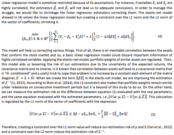
When we take statistical models to high dimensions (largenumber of predictors), we are moving to a world of sparsity. The general rule of this world is, roughly speaking, that when we have a large amount of predictors it is intuitive to think that only a group of them are relevant to describe our variable of interest.
In context of our problem, we have p as the number of assets that could be part of the portfolio. As we all are aware, not all stocks are good for the investor; therefore, he should not invest in all of them. The solution of (1), namely the Markowitz’ portfolio (MP), will assign a weight for each of the proposed assets. Some of them will be small, even pretty near to zero, if the associated securities are not relevant to the portfolio; nevertheless, the model will never be able to actually shift those small weights to zero even if is desired.
Here again, elastic-net outstands over the MP. When the linear regression has L1 and L2 norm constraints, besides of having the advantages exposed in 2.2, it will also select relevant variables. In pursuance of satisfying the norm constraint, some of the portfolio weights will go to zero in optimality, helping the investor to choose only some k of p assets that are statistically relevant.
Furthermore, as portfolios are rebalanced regularly, the investor need to assume some transaction costs each time he buys or sells shares. While the MP will force him to pay those costs for each of the p assets, disregarding if the asset has a high or small weight in the portfolio; the elastic-net solution with k<p assets reduces the transaction cost.
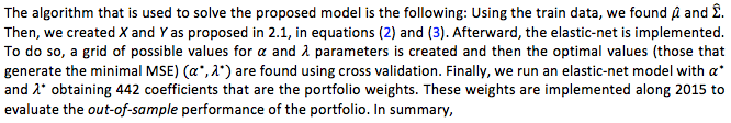
Table 1
Algorithm of implementation
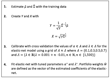
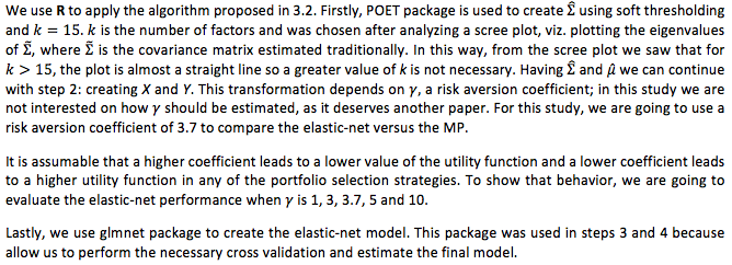
First of all, we are going to compare the performance of the elastic-net versus the traditional MP using a risk aversion coefficient of 3.7. The choice of this value will be discussed later.
As expected, the constraint over the L1 norm of the vector of coefficients in the elastic-net model helped us creating sparsity, as it is viewable in Table 2. The percentage of non-zero weights is 15.61% for the elastic-net compared to 100% of the MP. In this way, the elastic-net model shows that it can shift some weights to zero lessening the transaction costs.
Tabla 2
Percentage of non-zero weights for each strategy
|
Elastic-net |
MP |
Number of non-zero weights |
69 |
442 |
Percentage of non-zero weights |
15.61% |
100% |
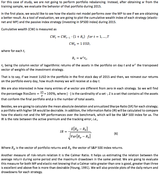
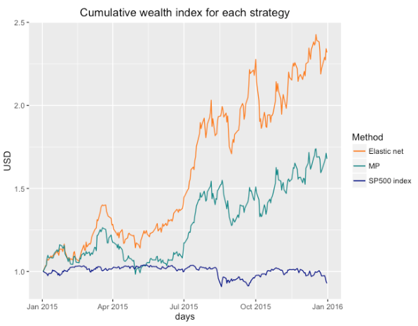
However, it is still important to see if having fewer assets in the portfolio yields better results. The plot of the cumulative wealth index is shown in Figure 1 where we compare the elastic-net portfolio, the MP and the CW investing directly in the S&P 500 index. During the chosen sample, the elastic-net model outstands over the others because, for the same level of risk aversion we obtain a higher plot of the CW. Figure 2 presents the same CW analysis with different levels of risk aversion.
It is viewable that starting with one dollar in each strategy and reinvesting profits daily, the elastic-net portfolio ends the year with 2.32 dollars while the MP ends with nearly 1.67 dollars.
Tabla 3
Portfolio performance indicators
|
Elastic-net |
MP |
Mean absolute deviation |
0.018 |
0.018 |
Annualized Sharpe Ratio |
|
1.971 |
Information Ratio |
3.564 |
4.106 |
Calmar Ratio |
7.303 |
3.241 |
In addition to the CW analysis, we obtained some portfolio performance indicators in Table 3. Firstly, we observed that when we measure risk of each portfolio based on mean absolute deviation, similar values were found, as it is 0.018 for both strategies. The annualized Sharpe Ratio has values greater than one proving a good performance over the risk free rate in MP and elastic-net; a greater SR for elastic-net shows that the model outstands over the MP. On the other hand, when we compare the portfolios versus the benchmark, both of them are desirable over the passive index strategy. It is important to mention that the MP showed a better information ratio. Lastly, we found that Calmar ratio for the MP is greater than 3, giving us excellent results. Furthermore, the Calmar ratio for the elastic-net is greater than 7 showing even a better performance.
Figure 1
Cumulative wealth index comparison between portfolio selection strategies
------
Figure 2
Cumulative wealth index using the elastic-net model for different type of investors
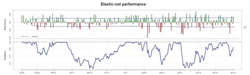
Considering these results, the elastic-net has a formidable behavior. Even though the MP scored a higher IR, the elastic-net has an excellent relation versus the S&P 500 index as well. It is important to mention that we are not taking into account transaction costs in any strategy. As the elastic-net has lesser assets, including transaction costs will reduce some performance indicators but not as much as it will for the MP; hence, creating a greater gap between the performances of both portfolios in favor of the elastic-net. Furthermore, we plotted daily returns and drawdowns for each strategy, as it is viewable in Figure 3 and Figure 4
Figure 3 Elastic-net performance.
Considering these results, the elastic-net has a formidable behavior. Even though the MP scored a higher IR, the elastic-net has an excellent relation versus the S&P 500 index as well. It is important to mention that we are not taking into account transaction costs in any strategy. As the elastic-net has lesser assets, including transaction costs will reduce some performance indicators but not as much as it will for the MP; hence, creating a greater gap between the performances of both portfolios in favor of the elastic-net.
Figure 4
MP performance
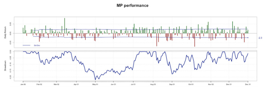
Furthermore, we plotted daily returns and drawdowns for each strategy, as it is viewable in Figure 3 and Figure 4. From these figures we can conclude that both of the time series have the same variance of their daily returns. We can see that the lower return for the elastic-net is -0.078 versus -0.071 for the MP during all 2015. Even though, in terms of drawdown, the maximum drawdown of the elastic-net is 18.5% while it is 22.2% for the MP; so the elastic-net has a better “worst case scenario” than the MP as the Calmar ratio showed in Table 3.
Finally, we analyze the behavior of elastic-net model when changes. Assuming that the risk aversion coefficient can be measured from 1 to 10 we evaluated the model with the values of 1, 3, 3.7, 5 and 10. From Figure 2 it is viewable that the CW is inversely proportional to the value of the risk aversion coefficient. As increases, we obtain lower curves of the cumulative wealth index
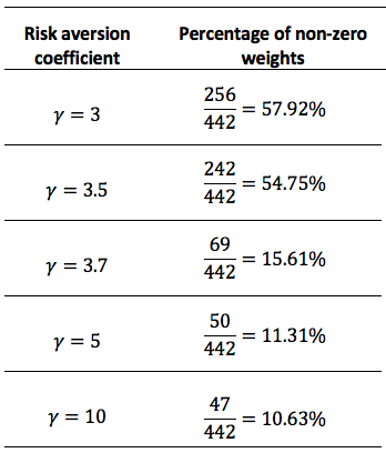
Table 4
Non-zero assets for elastic-net model for
different values of risk aversion coefficient
-----
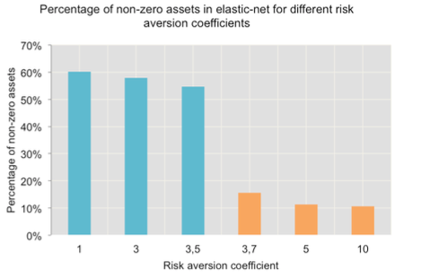
Figure 5
Non-zero percentages for elastic-net model and different values of γ
Two groups are clear in the plot, one for values of lesser than 3.7 and the other for values greater than 3.7. It is remarkable that for the group of the CW index line has more variance that the grouped lines of . Thus, we found that a risk aversion coefficient of 3.7 could be a good measure for an average investor and that justifies the value used for the comparison between MP and elastic-net.
Interestingly, when we evaluate the percentage of non-zero assets of each created portfolio when changes, the same two groups are easily recognizable. As Figure 5 shows, there are no significant changes in the percentage when the risk aversion coefficient changes between 1 and 3.7, and doesn’t change either when is between 3.7 and 10. Even though, the percentage is significantly different between the groups. When the percentage is near 50% and in other cases, it is approximately 10%. Real values are presented in Table 4. In any case, sparsity is present in the model; the elastic-net select assets and it is stricter as the risk aversion coefficient increases.
Some portfolio theories have been developed since Markowitz; nevertheless, some adjustments need to be done before implementing those theories in real data applications. It is impossible to invest without taking into account the randomness of the stocks prices in the market and then, portfolio selection models must include any control over parameter’s uncertainty. To cope this problem, we proposed a penalized linear regression model known as elastic-net; which regulate the L1 norm and L2 norm of the vector of weights. Despite of the addition of new constraints to the optimization problem, it gives better results in empirical applications due to the uncertainty of the expected returns and the covariance between them. We showed that the elastic-net model has a better performance over the MP during a year of evaluation, without rebalancing, and using only 5 years of daily data to estimate the parameters.
Furthermore, using the constrained model helped us controlling the estimation risk of its parameters and it also helped us selecting which assets should or should not conform the portfolio.
The elastic-net model changes accordingly to the risk aversion coefficient and it remains for future works how to estimate an adequate risk aversion coefficient. It will be also interesting to study model’s performance when some constraints are added; not the ones that control parameter uncertainty but portfolio constraints that are common in real financial applications. For instance, restricting the minimal percentage of health care assets in the portfolio. Some methods that have been proposed to work with sparsity, like non-parametrical graphical models, (e.g. Lafferty et al., 2012) can be applied to the portfolio selection problem and thus, as future work they could be compared with the elastic-net.
Markowitz, H. (1952). Portfolio Selection. The Journal of Finance 7 (1): 77–91.
Li, J. (2015). Sparse and stable portfolio selection with parameter uncertainty. Journal of Business & Economic Statistics 33 (3): 381–92. doi:10.1080/07350015.2014.954708.
Fan, J., Zhang, J., and Yu, K. (2012). Vast portfolio selection with gross-exposure constraints. Journal of the American Statistical Association 107 (498): 592–606.
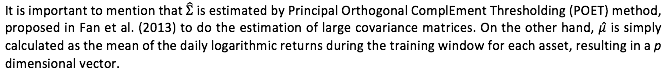
Fan, J., Liao, Y., and Mincheva, M. (2013). Large covariance estimation by thresholding principal orthogonal complements. Journal of the Royal Statistical Society: Series B (Statistical Methodology) 75 (4): 603–80.
Lafferty, J., Liu, H., and Wasserman, L. (2012). Sparse nonparametric graphical models. Statistical Science 27 (4): 519–37.
Young, T.W. (1991). Calmar ratio: A smoother tool. Futures 20(1), 40.
DeMiguel, V., Garlappi, L., Nogales, F. J., & Uppal, R. (2009). A generalized approach to portfolio optimization: Improving performance by constraining portfolio norms. Management Science, 55(5), 798-812.
Shen, W., Wang, J., & Ma, S. (2014, July). Doubly Regularized Portfolio with Risk Minimization. In AAAI (pp. 1286-1292).
1. Master student. Industrial Engineering Department. University of los Andes, Bogotá, Colombia. Email: dh.segura10@uniandes.edu.co
2. Professor. Industrial Engineering Department. University of los Andes, Bogotá, Colombia. Email: cf.valencia@uniandes.edu.co