ISSN 0798 1015

Vol. 40 (Number 20) Year 2019. Page 1

Assessing Promotional Effectiveness in Retail Industry through Estimation of Sales Components

Evaluación de la efectividad promocional en la industria minorista a través de la estimación de los componentes de ventas

DAS, Biswajita 1; BISWAL, Saroj Kanta 2 & MISHRA, Soumya 3

Received: 12/11/2018 • Approved: 31/05/2019 • Published 17/06/2019

Contents

1. Introduction

2. Methodology

3. Major Results & inferences

4. Summary & conclusion

Bibliographic references

1. Introduction

Retail is so dynamic and complex industry that multiple brands of a same product category compete for customers with a varying promotional calendar in different seasons.  At any given point of time a big retailer may be dealing with more than a hundred thousand products coming from various categories and brands. Retailers are concerned about which product is being sold the most or which product has high response during promotion to be able to plan their marketing activities and floor designing. Such questions could be adequately answered when retailers have an overview of the key factors driving the sale of a particular product and how much is the incremental benefit accrued to their promotions. Thus, sale of a product could be expressed as a function of three major components namely – incremental sale from promotion, seasonal sale and cannibalised sale due to competitors.

In the current high-competition retail environment firms are under greater pressure to demonstrate the economic return from marketing expenditures, the need for a new measurement standard has emerged. By studying whether marketing expenditures generate sales above the baseline, the businesses are evaluating whether their various marketing activities are generating increases in sales and profitability. 

 This study is focused on estimating the key metrics of a product sale, namely - Base Sales, Incremental Sales, Adjustment Factor (includes seasonality & any other extraneous factors) and Cannibalized Sales. This will also discuss a few methods that help to devise the decision rules for competitor set identification within products.

1.1. Data Plan & Preparation

With the objective of estimating the key metrics - Baseline Sales, Incremental Sales, Adjustment Factor (includes seasonality & any other extraneous factors) and Cannibalized Sales – the study used two years of transactional history of sales data of a national grocer at the UPC (unique product code) level for each product of the 104 weeks. Since not all products were on promotion for 104 weeks and not all products were sold for all 104 weeks, we had a challenge to deal with low transactional history for each product. 

Table 1

2. Methodology

2.1 Challenges and Assumptions

The study made certain assumptions to counter challenges related to data and promotional cycle as below:

1. Week without any sales: such weeks were replaced with zero sales or were excluded.
2. Lack of data on promotion details: Same set of products could be sold in multiple stores but only few of the stores would be on promotion. In such cases, even if one store was on promotion, it was assumed that all the stores were in promotion for all computational purposes.
3. Identification of competitor set: For the identification of direct competitor set of a product, average prices were compared to arrive at the closest direct competitor. Though this method has been widely used but suffers from accuracy and entirely depends on the price of the product, due to lack of adequate data, other suitable methods were ignored. The details of this approach will be discussed in the next section.

2.2 Analytical Approach

2.1.1. Data processing for model development

 For any modelling, it is very important to create the factual dataset. Sometimes we do not get data in a readymade form to perform the require modelling exercise. The data from different sources of data tables need to be integrated and summarised to create the master dataset.

2.1.2. Defining the sales components

Sales value of a product can be expressed as a function of incremental sales, seasonal/ adjustment factors and cannibal sales i.e.

Product Sales = α (intercept) + →Baseline Sales

β1 * Promo Flag + →Incremental Sales

β2 * Seasonal Dummies + →Adjustment Factor

β3 * Previous week unit sale + →Adjustment Factor

β4 * Competitors units sales (on Promotion) + →Cannibalized Sales

ε (Residual term)

2.1.3. Segmenting the population for modelling

 Any sale in absence of these influences is called as base sale. A rich historical data not only helps to build more robust models, but also allows the choice of technique from the wide variety of options available. However, in reality the data might be insufficient or lacks history for any robust modelling exercise. This restricts the use of modelling techniques to a few that suits the data and the best possible one is chosen. In this study cases of data with not more than 2 years of transactional history & promotion details across product were seen. It is a fact that not all products are sold throughout the year neither would all the products be on promotion all the year round. This is thus a clear case of less history and limited information. 

 To cope up with the variation in availability of historical data & promotion details across multiple products, the base data was segmented in to the below five categories. This will not only help capture the information for each segment but also help in building a model that would be specific to the relevant segment’s characteristics.

Table 2

2.3. Direct Competitor Set Identification

As mentioned above promotional and seasonal sales could be represented as dummy variables in the regression model. However, to calculate the cannibal sales, we would need a profound understanding of competitor set of products. We know competitors could be within the category or the brand. 

There are various methods that could be used to identify the set. Among them the following methods are widely used:

1. Price based selection method, 
2. Product switching method
3. Direct correlation method.

2.3.1. Price based selection method

The price based selection is based on similar price for products. In other words products priced similarly within a category may be considered as competitors. One can always decide upon what hierarchy level they would want to form the competitor set. This method comes handy when not all products have a good transactional history, but have been sold in some point of time and thus their average prices could be compared. This is an approximate but useful method.

2.3.2. Product switching method

Product switching is a correlation based method. The target product unit sale is correlated with the unit sales of other products present in the category. Products having high correlation with the target product are considered as its competitor. However, this method has a caveat, i.e. the competing products should have sales for the same time frame for a fare comparison. In case, the two products are sold in different time points, this method becomes difficult to apply.

2.3.3. Direct correlation method

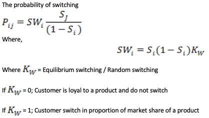
This method calculates the probability of switching of a given target product by other products present in the same sub category. Thus, products having higher switching probabilities are considered competitors for the given target product. However, this method also faces the same problem as product switching.

Thus, when all products are not sold across all the weeks, it becomes a limitation for “product switching” and “direct correlation” methods. In such cases “price based selection” proves to be a better option. Once promo & season flags are created and the competitor sets are identified, we are through with our master dataset creation. This master data then could be divided into segments for the modelling exercise to be implemented.

2.4. Sale Components estimation modelling

There are many techniques that have been used to compute the sales components. To name a few are - Localized Regression, Mixed Regression and OLS Regression. Now let’s scrutinize the advantages and dis-advantages for each of the above techniques.

Localized regression is a non-parametric estimation method for the computation of the predicted values. This method, however, does not produce estimates for the predictor variables. This becomes a challenge to compute any of the component metrics separately. Also, the computational time is more as compared to any other technique.

 Mixed regression is another useful method. However, the challenge lies in measuring the cannibalization effect for each product. The reason being mixed regression reports the contribution of both fixed and random effects, and random coefficient are not populated for the competitor products. As a consequence, this method again faces a setback when the objective is to segregate the predicted sales into its components.

 In such a scenario, OLS regression proves to be optimal method due to its simple and explicit computation of parameter estimates for thousands of products and for various segments of products in the data. OLS can be applied to products having at least 5 week of history for the above reasons. 

 The model equation is explained as below:

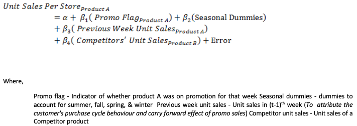
The idea of having unit sales per store as dependent variable stems from the fact that the trend of the unit sales is different across the two years, which is mainly due to number of stores the product was sold. Also to capture this trend in the analysis, unit sales is normalized by dividing with the number of stores the product is sold. 

For products having transaction history less than 5 weeks, a look-alike procedure could be adopted. This procedure basically correlates products with less history to those with at least 5 weeks of history on the basis of similar sales trend. The assumption of lookalike procedure is that the sale of products with less than 5 weeks of history would be distributed into its components similar to the propositions their look-alike products (with at least 5 weeks of history). 

3. Major Results & Inferences

Any retailer would be curious to know about the performance of the product. In other words when does a particular product draw customers’ attention? Say a particular product is sold mostly during promotion. OR there is no effect of any marketing strategy for a product, since it gets sold as it is, hence a popular product. These queries get clarified more when we look into the stats for the components contribution.

Table 3

The results of the OLS regression models showed that the Promo flags, seasonal dummies, competitor unit sales, previous week sales were found to be the statistically significant drivers of unit sales of a given product. 

 Thus the steps involved in the sale computation process viz., identifying the competitor set, segmentation and choosing the correct modelling method would result into estimation of product sales into Baseline Sales, Incremental Sales, Adjustment Factor, and Cannibalized Sales components at each product level. For effective use of the results for business purposes, adjustment factor was redistributed to Baseline and Incremental sales to account for external effects. Incremental benefits due to the promotions were expressed in percentage terms which were in the range of 2% to 15% for various products. The incremental benefits were observed to be higher for the perishables (12-15%) compared to other product categories. 

 The above results would help to measure the increment in sale due to promotion run for a particular product for a given period. The results can also help the business to understand what components contributes the most for a product sale in a given week in order to devise appropriate marketing strategies.

4. Summary & Conclusion

In the era of cut-throat competition in the retail industry it is very critical to gauge the effectiveness of marketing activities and the impact of competitor activities. Hence estimating the sale components through a scientific approach is a critical exercise from the retail marketing perspective. 

 The analyses were carried out using the 5-stage analytical framework including data aggregation, model building and validation. OLS regression was employed to build models at product-week level for computing baseline, incremental and cannibalized sales along with adjustment factors. Due to the variability in data history and promotion calendar, the products were divided in to 5 different segments based on the data/information availability in terms of presence or absence of promotion, availability of history and competitor details. Models were built independently for each segment. Competitors of a product were identified using price proximity approach among the alternative methods such as direct correlation method, product switching behaviour method, etc.

 The results of the OLS regression showed that Promo flags, seasonal dummies, competitor unit sales, previous week sales were found to be the statistically significant drivers of unit sales of a given product. Overall, the incremental benefits due to promotion were found to be in the range of 12-15% varying across different product categories.

 The study could further be improved with the help of data around product hierarchy and specific promotion details. Such data would have provided comparison of effectiveness of different promotion activities.

Bibliographic references

1. David A. Dickey, “PROC MIXED: Underlying Ideas with Examples”; NC State University, Raleigh, NC

2.Kurt Jetta, TABS Group, Shelton, Connecticut, Erick W. Rengifo , “A Model to Improve the Estimation of Baseline Retail Sales”; Fordham University, New York, New York

 3. Robert C. Blattberg, Kellogg Graduate School of Management, Northwestern University, Byung-Do Kim, ”Defining Baseline Sales in a Competitive Environment”; College of Business Administration, Seoul National University, Jianming Ye Graduate School of Business, 'Ihe U n i d t y of Chicago

 4. Rolf Steyer, “Conditional Expectations: An Introduction to Concept and its Applications in Empirical Sciences”

 5. Wendy Lomax, Kathy Hammond, Robert East and Maria Clement, “The measurement of cannibalization”

 6. William S. Cleveland and Clive Loader, “Smoothing by Local Regression: Principles and Methods”; AT&T Bell Laboratories, 600 Mountain Avenue, Murray Hill, NJ07974, USA

1. Research Scholar, Faculty of Management Sciences, Siksha O Anusandhan (Deemed to be University), das.biswajita@gmail.com

2. Associate Professor, Faculty of Management Sciences, Siksha O Anusandhan (Deemed to be University), sarojkantabiswal@soa.ac.in

3. Assistant Professor, Faculty of Management Sciences, Siksha O  Anusandhan (Deemed to be University), soumyamishra@soa.ac.in