ISSN 0798 1015

Vol. 40 (Number 14) Year 2019. Page 15

The effects of changes in oil prices on the russian economy

Los efectos de los cambios en los precios del petróleo en la economía rusa

SYZDYKOVA Aziza 1; TANRIÖVEN Cihan 2; NAHIPBEKOVA Symbat 3 & KURALBAYEV Almaz 4

Received: 18/12/2018 • Approved: 23/03/2019 • Published 29/04/2019

Contents

1. Introduction

1. Introduction

Oil is the most important non-renewable energy resource in the world. It is used as an intermediate good in textile, defense and transportation industries as well as a raw material in the world economy. Therefore, oil price changes are quite relevant to the world economy. Oil price changes especially affect the oil-dependent countries (Alagöz et.al., 2017: 144).

Oil price changes effect oil exporting and importing countries very differently. These effects can be either on the supply and demand sides and they can be direct or indirect. Accordingly, a high oil price means increased revenue for an oil exporting country whereas it means cost increases, decreased production and decreased exports as well as impaired economic growth for an importing country (Abeysinghe, 2001: 149). The growth effect of the high oil prices for an exporting country may vary when its slowing effect on the importing countries is considered. A decreased demand of a net energy importing country also decreases the export rates of an exporting country. This causes a negative effect on the economic growth (although not so sharp in the oil exporting countries). Although high oil prices are expected to cause a positive economic effect on the energy exporting countries, its effect proves to be ambiguous when trade relations are considered (Korhonen and Ledyaeva, 2010: 849). Oil revenues contribute greatly to the economic performance of developing, oil exporting countries as a financial source for investments. Thus, oil price shocks create dramatic effects on the economic growth of these countries (Köse and Baymaganbetov, 2016).

The extent of the effect of high oil prices on an economy depends in general on the share of oil consumption in the relevant economy (Schneider, 2004). Russia is one of the most important energy producers of the world with its 60 billion barrels of oil and 150 trillion cubic meters of natural gas reserves. She is also the biggest energy exporter besides OPEC members. She is the second biggest oil exporter after Saudi Arabia and the biggest natural gas exporter.

This study examines how and to what extent the raw oil price affects the macroeconomic variables of Russia (industrial production, inflation, exchange rates, and interest rates). This study is comprised of four sections. The first section discusses annual oil price changes and the effect of these changes on the economy of Russia. The second chapter includes the literature review and the third explains the data set used and the econometric method employed. Lastly, the analysis results are explained and concluded.

2. Oil Price Changes and the Economy of Russia

Until today, increases in oil price have caused serious effects on the global economy. Oil price shocks, and after effects of these shocks were imprinted on the memories. Especially in the 1970’s and 1980’s, acute increases in oil price devastated many national economies and caused negative effects such as high inflation and high interest rates. These price increases showed their effects on the developed countries as deep economic recessions (Syzdykova, 2017). In Figure-1, fluctuations in the international oil price during the 1950-2018 period is presented.

Figure 1
Fluctuations in the Oil Price during the 1950- 2018 Period

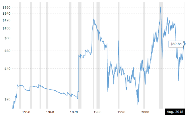
Source: http://www.macrotrends.net/1369/crude-oil-price-history-chart

Since 1970, the world economy has experienced four major oil price shocks. The first shock was triggered by the OPEC’s decision to cut oil production. Whereas the barrel price of oil was 11.24 dollars in 1972, it increased to 20.18 dollars in 1975 (80% increase). The second shock was triggered by the Iran-Iraq war in the 1980’s. Oil price increased from 19.67 dollars to 53.74 dollars (173% increase). The third shock was triggered 10 years later by Iraq’s occupation of Kuwait. Oil price increased from 16.62 dollars to 24.55 dollars (48% increase). The fourth one was experienced because of the U.S.A.-Iraq war in 1999-2000 and increased geopolitical tensions in the Middle East. Oil price increased from 11.27 dollars to 15.90 dollars in 1998, and to 26.72 dollars in 2000.

Oil price showed a rapid increase in the international markets from 2003 to 2008. Nevertheless, after the 2008 crisis, which was triggered by the mortgage crisis in the U.S.A. and turned into a financial one, the oil price dropped to 60 dollars level. But it started to rally again with a rapid growth trend in the developing countries and with the production loss expectation following the Arab Spring. Thus, prices that soared up to 160 dollars in the world oil market created a trend that cruised above 100 dollars level from 2010 to 2014 (OPEC, 2014). 

From June 2014 on, oil price assumed a sharp and continuous falling trend again and dropped to 56.32 dollars in April 2015 (Davig et.al. 2015: 6). Oil price didn’t stay at this level and dropped to 30 dollars in February 2016. This had a very negative effect on Russia. Because oil production cost in Russia is about 76-77 dollars whereas it is about 20 dollars in the Middle East (Göçer and Bulut, 2015). Any price under this level means a losing bargain for Russia. The Russian Government collects approximately half of her tax income from oil and natural gas sales. Barrel price of oil should be about 100 dollars level for the Russian budget not to produce a deficit (BBC, 2015). But, as seen in Figure-1, barrel price of the oil was 69.84 dollars in August 2018.

When recent sharp oil price falls are considered from the perspective of Russia, an economic stagnation seems inescapable. Russia’s macroeconomic indicators and international oil prices in 2000 are shown in Table 1.

Table 1
Russia’s Macroeconomic Indicators and Oil Price

Source: World Bank, 2018

Since 2000, together with an increase in oil price, GDP of Russia greatly improved and macroeconomic indicators such as production, employment and exports started to present a dependent relationship with the oil sector. In Table 1, one can see that in years that oil price rises Russia obtains high levels of economic growth, whereas she shows stagnated growth levels in years in the which oil price falls. The financial crisis of 2008 caused a drop in the oil price and the volatility of oil prices in this period disrupted the price stability.

In 2013, Russia has earned 50.2% of her national income from oil and natural gas sales. When the barrel price of Brent oil dropped from 110 dollars in 2014 to 47 dollars in January 2015, Russia suddenly faced with the risk of an economic crisis. This caused a serious concern when the over dependency of the economy of Russia on oil prices is considered. The statement announced by the Central Bank of Russia in January 2015 explained that hot money escaped from Russia in 2014 due to falling oil prices and the damage caused by this in the economy of Russia amounted up to 151.5 billion dollars (Göçer and Bulut, 2015).

Together with the falling oil price, the ruble is also devalued. Russia went through hard days and her international credit rating have been taken under negative watch. First international rating institution that declared it had taken Russia’s credit rating under negative watch was Standard & Poor’s (S&P) on December 23, 2014. After that, Fitch dropped the rating of Russia to BBB- on January 12, 2015, and lastly Moody’s dropped Russia’s rating from Baa2 to Baa3 on January 16, 2015, and that was the lowest rating for investment. Subsequently, Russia Stock Market lost its value by 44%.

The relation between the oil price changes and value of ruble is given in Figure 2.

Figure 2
The interaction between oil price and the value of Ruble

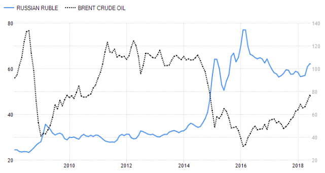
When Figure 2 is examined, a general trend can be observed. When oil price starts to rise Russian ruble gains value, but when oil price starts to fall, Russian Ruble also loses its value. For example, in 2014, ruble experienced a 46% fall against the dollar and became the worst performing currency.

When oil price falls, ruble devalues greatly. This leads to an increase in the real effective exchange rate and effects Russia’s competitive power and her exports negatively. Low oil price also affects the risk perception, CDS spread and borrowing costs of Russia.

3. Literature Review

The literature review constituted the basis of variable, method and model preferences for the econometric analysis. When the economics literature is reviewed, one can spot many empirical studies that prove a negative relation between the oil price and macroeconomic activity.

Hamilton (1983:228-248), Gisser and Goodwin (1986:95-103), Burbidge and Harrison (1984:459-484), Mork (1989:740-744) and Hooker (1996:195213) studied the relationship between the oil price and GDP. The common point of all these studies is that all show that oil price changes cause the economic recession in the U.S.A.

Although not many, there are also studies that show a positive, weak and insignificant relation between oil price and economic growth. Besides the studies of Tabata (2006), Prasad et.al. (2007), Farzanegan and Markwardt (2009), and Berument et.al. (2010) that shows the positive effect of oil price shocks on the economic growth, the studies of Chang and Wong (2003), and Ayadi (2005) shows the existence of statistically insignificant relations between the relevant variables. Studies of Asafu-Adjaye (2000), and Barsky and Kilian (2004) also shows that oil prices have a very weak effect on the economic growth.

Blanchard & Gali (2007) states that oil prices were not a significant cause of economic fluctuations in the last decade. Authors explained the mild effect of a high oil price on the inflation and economic activity by four factors. These are the non-existence of consequent negative shocks, relatively small share of oil in the production process, the elasticity of labor market and improved monetary policies. On the other hand, Segal (2007) explains the slowing effect of high oil prices on the world economy during the 2000’s for various reasons. More important ones are relative unimportance of high oil prices when compared with the perceived importance, and the prevention of pass-through effect of high oil prices on the core inflation with tight monetary policies. But these results are usually attributed to oil and energy importing countries. On the contrary, energy exporting countries are expected to benefit more from high prices. Improved terms of trade and increased export revenues of these countries are used both for more production and for investments. For example, Rautava (2004) showed clearly that increased oil revenues cause great increases in Russia’s GDP.

The differences found in the results of these studies can be explained by the additional variables included in the studies, differences in time periods and data frequencies, and different econometric methods employed.

Table 2
A summary of empirical studies on Russia

4.1. Data Set and Model

This study used the barrel price of Brent crude oil, industrial production index, inflation, 3-month deposit interest rate, and real effective exchange rate values belonging to January 2010-April 2017 period to examine the macroeconomic effects of oil price changes on the economy of Russia. We took the logarithm of all series except interest rate. Seasonal effects are removed from the series using Tramo/Seats method and Eviews 9 package program. Oil price series are taken from the official website of Energy Information Administration (EIA), and data of the other series are taken from IMF, IFS database.

We examined the effect of oil price changes on every macroeconomic indicator of Russia separately. In this context, we estimated four different regression models with different dependent variables.

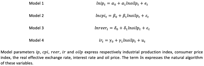
We selected these models because the variables used in these models are the most important macroeconomic indicators and an oil exporting countries are mostly affected by the oil price changes through these channels.

4.2. Research Method

In this study, we used the VAR method to study the effects of oil price changes on the economy of Russia. Vector Autoregressive (VAR) method is developed by Sims (1980) and uses Granger causality test model (Granger, 1969) as its basis. It helps to analyze the interrelation between the selected series. VAR models consist of the regression of the current and past values of every variable and they show the dynamic relationship between these variables.

VAR models are used primarily to study the relation between the macroeconomic variables and to study the dynamic effects of random (accidental) shocks on the system created by these variables. VAR modeling based on the Granger Causality Test analyzes the relation between the variables using variance decomposition and the impulse-response functions. VAR modeling is very sensitive to the selected lag length. In the VAR analysis, the lag lengths of the variables, which will be included in the model, should be selected to capture the dynamic relations among these variables. Furthermore, VAR models make strong forecasts possible by including the lagged values of dependent variables (Kumar et.al., 1995: 365).

A standard VAR model can be expressed as follows:

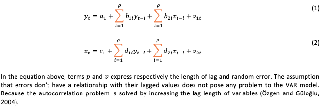
As known, it is quite hard to interpret the resulting coefficients from the estimated VAR model individually. There are two ways to overcome this hardship: i) the impulse-response analysis and ii) variance decomposition method.

Therefore, the VAR model we used in this study is analyzed with the impulse-response functions and variance decomposition method. By using the impulse-response analysis, we could determine the response that will be given by all the other variables to a change in any variable and how long will it take to find the balance after that shock. By using variance decomposition analysis, we can determine how much change in a series is caused by the changes in the relevant variable and how much change is caused by the changes in the other variables.

5.1. Results of the Unit Root Test

Granger and Newbold (1974) showed that we can encounter with the fake regression problem when non-stationary time series are used. Since then, it has become a standard procedure for studies which use time series to analyze the stationarity of the series. When we call a time series stationary, we mean a constant variance and median value through time and the dependency of the covariance of the variables of two lagged time periods to the lag between variables but not to the time (Gujarati, 1995:712).

The most commonly used method to analyze the stationarity of time series is ADF unit root test. In this study, we used the expanded Dickey-Fuller and Phillips-Perron unit root tests to analyze the stationarity. Results are shown in Table 3.

Table 3
Results of ADF Unit Root Test

As seen in Table 3, the results of ADF and PP tests show that the first order differences of all variables don’t include a unit root. Critical values of t statistics for ADF and PP tests show that first order difference of all variables is stationary at the 1% significance level. Therefore, short-term VAR model should include the first order difference of the variables.

5.2. Determination of the Lag Length

One of the most important decisions to be made for the VAR analysis is the determination of lag numbers of the series that will be included in the model. We used two criteria, namely Akaike information criterion (AIC) and Schwarz criterion (SC) to determine the lag lengths required for the VAR analysis. The final decision is given on the Akaike information criterion.

Table 4
Determination of optimum lag length

As seen in Table 4, the optimum lag number is selected as 3 based on all three criteria (LR, FPE, and AIC).

5.3. Results of the Causality Test

The results of the Granger causality test, which is performed to determine the directionality of the causality between the variables, is given in Table 5 below. Thus, we found that the oil prices are the cause of the changes in macroeconomic indicators such as inflation, industrial production index and real exchange rate. In contrary, we failed to refute the  hypothesis which claims that oil prices are not the Granger cause of the short-term interest rates in Russia. Hence, oil prices are not the Granger cause of the interest rates. On the other hand, Granger causality relation is unidirectional and moves from oil prices to the macroeconomic variables. We failed to find any directional causality that moves from the aforementioned variables to the oil prices.

Table 5
Results of the Granger causality test

5.4. Results of the Impulse-Response Analysis

The impulse-response function is a method used to determine the directionality and volume of the reaction given by the series included in the VAR model to the shocks in the error terms. And the variance decomposition analysis is used to determine the sources of a change in a series. The impulse-response function is also used to determine how the other series react when a shock is applied to one of the series. Figure 3 shows the results of the impulse-response function.

Figure 3
Results of the impulse-response function

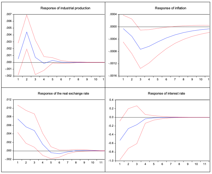
We can see that the greatest response to an oil price change within standard deviation is given by the inflation variable. The response given by the inflation variable to an oil price change within standard deviation is negative for a year and is stable. The response of the industrial production index to the oil price changes is positive for the first 4 months, but after the 5th month it turns to negative. Real effective exchange rate shows a positive response for the first 5 months but starts to show a negative response in the following two months. The response of interest rate is negative for the first 5 months but after that, the response disappears.

5.5. Results of the Variance Decomposition

Variance decomposition, which is used to evaluate the direct and indirect effects among the variables, calculates the percentage of the sources of shocks experienced in one of the variables. This shows how much of a change in the variables are caused by them and how much of it is caused by the other variables (Özgen and Güloğlu, 2004: 101). The results of the variance decomposition are presented in the following tables.

When we examined the results of the variance decomposition of the real exchange rate variable (Table 6), we can see that its self-explanatory power is high for the first 4 months. While the explanatory power of oil prices for the real effective exchange rate is 9% for the first 3 months, after the 3rd month it rises to 12%. Industrial production index and the interest rate have the highest explanatory power for the changes in the real effective exchange rate, respectively 5.3% and 4.5%.

Table 6
Variance decomposition of the real
effective exchange rate variable

This table gives the variance decomposition of the inflation variable for 12 periods. We can see that the self-explanatory power of this series is high for the first two months. But starting with the 3rd month, 6% of the changes in the inflation variable can be explained by the real exchange rate and 5% of it can be explained by the oil price. But the important point is not to confuse it with the concept of shock or in other words an unexpected movement in the series. But the industrial production index and interest rates have a very insignificant explanatory power for the changes in the inflation variable.

Table 7
Variance decomposition
of the inflation variable

When the results of the variance decomposition of the industrial production index are analyzed (Table 7), we can see that the changes in the industrial production index can be explained completely by its own dynamics. After the second month, 11% of the change can be explained by the changes in the oil price. Another finding is that starting with the second month the real effective exchange rate can explain the 6% of the changes in the industrial production index.

Table 8
Variance decomposition of the
industrial production variable

As seen in the table, the changes in interest rate can be explained by the variable itself especially in the first month. After the second month, 7% of the changes can be explained by oil price and 3% of it can be explained by the industrial production index. The explanatory powers of the real exchange rate and inflation rate are low. This result proves that interest rates are dependent on oil price and industrial production index.

Table 9
Variance decomposition of
the interest rate variable

In 2017, Russia ranked as the 11th biggest economy in the world with her 144 million population and 1,562 billion dollars GDP. Russia earns 50.2% of her national income from oil and natural gas sales. When the barrel price of Brent oil dropped from 110 dollars at the beginning of 2014 to 47 dollars in January 2015, she faced a serious economic crisis threat. Therefore the economy of Russia is very dependent on oil.

If economy policymakers can properly identify the interrelations between macroeconomic indicators and effects of external variables on these indicators, this contributes greatly to the economic and political stability. This study examined the effects of oil prices on the macroeconomic activities in Russia using VAR analysis and data from January 2010-April 2017 period. Furthermore, we performed Granger causality analysis to examine the causality relation between the variables.

According to the results on the impose-response function performed under the VAR analysis, an oil price shock within the limits of standard deviation creates different effects on macroeconomic variables. The greatest response can be observed in inflation. The response of the inflation variable to an oil price shock within the limits of standard deviation is negative for a year and is stable. The response of the industrial production index to the oil price shocks is positive for the first 4 months, but after the 5th month response is lost. Real effective exchange rate shows a positive response for the first 5 months but starts to show a negative response in the following two months. The response of interest rate is negative for the first 5 months but after that, the response disappears. According to the results obtained from the variance decomposition, the oil price has a high explanatory power on the macroeconomic changes.

The results of Granger causality analysis showed a unidirectional causality stemming from oil price and affecting all other variables. This result proves that, in the short term, oil price is the Granger cause of inflation, industrial production, real exchange rate, and interest rate.

In conclusion, an important point is that 80% of the energy products of Russia is exported to the developed countries in Europe. Future contains many prospects for the use of renewable energy sources. Thus, if Russia wants to mitigate her dependency on Europe for energy exports and to solve the problems with the transit countries, she has to develop balancing policies for the east-west energy market.

Abeysinghe, T. (2001). Estimation of Direct and  Indirect  Impact of Oil Price on Growth, Economics Letters, 73, 147–153.

Alagöz, M., Alacahan, N. D., & Akarsu, Y. (2017). Petrol Fiyatlarının Makro Ekonomi Üzerindeki Etkisi-Ülke Karşılaştırmaları İle Panel Veri Analizi. Sosyal ve Ekonomik Arastırmalar Dergisi, 19(33), 144-150.

Asafu-Adjaye, J. (2000). The relationship between energy consumption, energy prices and economic growth: time series evidence from Asian developing countries. Energy economics, 22(6), 615-625.

Ayadi, O. F. (2005). Oil price fluctuations and the Nigerian economy. OPEC review, 29(3), 199-217.

Barsky, R. B., & Kilian, L. (2004). Oil and the Macroeconomy since the 1970s. Journal of Economic Perspectives, 18(4), 115-134.

Benedictow, A.,  Fjærtoft, D. ve Løfsnæs, O. (2010).  Oil  Dependency of the Russian Economy: An Econometric Analysis,  Statistics Norway, Research Department, Discussion Papers, No. 617.

Berikan, M., & Hüseyinli, T. (2017). Petrol fiyatlarındaki düşüşün Rusya ekonomisi üzerine etkileri. İktisadi Yenilik Dergisi, 4(2), 30-45.

Berument, M. H., Ceylan, N. B., & Dogan, N. (2010). The impact of oil price shocks on the economic growth of selected MENA countries. The Energy Journal, 149-176.

Blanchard, O. J., & Gali, J. (2007). The Macroeconomic Effects of Oil Shocks: Why are the 2000s so different from the 1970s?(No. w13368). National Bureau of Economic Research.

Brown, S. P., & Yuecal, M. K. (1999). Oil prices and US aggregate economic activity: a question of neutrality. Economic and financial review-federal reserve bank of Dallas, 16-23.

Burbidge, J., & Harrison, A. (1984). Testing for the effects of oil-price rises using vector autoregressions. International Economic Review, 459-484.

Davig, Troy, Nida Cakir Melek, Jun Nie, A. Lee Smith, and Didem Tuzemen (2015), "Evaluating a Year of Oil Price Volatility," Federal Reserve Bank of Kansas City, Economic Review, Third Quarter 2015.

Deniz, M. H., & Sümer, K. K. (2015). Petrol Fiyatlarındaki Oynaklığın Dış Ticaret ve Milli Gelir Üzerindeki Etkisi: Seçilmiş Bazı Avrasya Ekonomileri Üzerine Bir İnceleme. In International Conference On Eurasian Economies.

Farzanegan, M. R., & Markwardt, G. (2009). The effects of oil price shocks on the Iranian economy. Energy Economics, 31(1), 134-151.

Ghalayini, L. (2011). The  Interaction between Oil Price  and Economic Growth, Middle Eastern Finance and Economics, 13, 127-141.  

Gisser, M., & Goodwin, T. H. (1986). Crude oil and the macroeconomy: Tests of some popular notions: Note. Journal of Money, Credit and Banking, 18(1), 95-103.

Göçer, İ., & Bulut, Ş. (2015). Petrol Fiyatlarındaki Değişimlerin Rusya Ekonomisine Etkileri: Çoklu Yapısal Kırılmalı Eşbütünleşme ve Simetrik Nedensellik Analizi. Çankırı Karatekin Üniversitesi İİBF Dergisi, 5(2), 721-748.

Granger, C.W.J. (1969).  Investigating Causal Relations  by Econometric Models and Cross-Spectral Methods, Econometrica, 37, 424-438.

Hamilton, J. D. (1983). Oil and the macroeconomy since World War II. Journal of political economy, 91(2), 228-248.

Hooker, M. A. (1996). What happened to the oil price-macroeconomy relationship?. Journal of monetary Economics, 38(2), 195-213.

Ito, K. (2010). The impact of oil price volatility on macroeconomic activity in Russia (No. 2010, 5). Economic analysis working papers. https://www.econstor.eu/handle/10419/43420 Erişim: 08.08.2018

Korhonen, L. A, & Ledyaeva, S. (2010). Trade linkages and macroeconomic effects of the price of oil. Energy Economics, 32, 848–856.

Kose, N., & Baimaganbetov, S. (2015). The asymmetric impact of oil price shocks on Kazakhstan macroeconomic dynamics: A structural vector autoregression approach. International Journal of Energy Economics and Policy, 5(4), 1058-1064.

Kumar, V., Leone, R. P., & Gaskins, J. N. (1995). Aggregate and disaggregate sector forecasting using consumer confidence measures. International Journal of Forecasting, 11(3), 361-377.

Mork, K. A. (1989). Oil and the macroeconomy when prices go up and down: an extension of Hamilton’s results. Journal of political Economy, 97(3), 740-744.

Özgen, B. F. ve Güloğlu, B.,  (2004).  Türkiye’de İç Borçların İktisadi Etkilerinin VAR Tekniğiyle Analizi, METU Ssudies in Development, vol. 31, s. 93-114.

Prasad, E. S., Rajan, R. G., & Subramanian, A. (2007). Foreign capital and economic growth (No. w13619). National Bureau of Economic Research.

Rautava, J. (2004). The Role of Oil Prices and the Real Exchange Rate in Russia’s Economya  Cointegration  Approach,  Journal of Comparative  Economics, 32, 315–327.

Reynolds, D.B. ve Kolodziej, M.(2008). Former Soviet Union Oil Production and GDP  Decline: Granger  Causality  and  the Multi-Cycle  Hubbert  Curve, Energy Economics, 30(2), 271-289.

Schneider, M. (2004). The impact of oil price changes on growth and inflation. Monetary Policy & the Economy, (2).

Segal, P. (2007). Why do oil price shocks no longer shock?. Working paper. OIES paper: M35 , Oxford Institute for Energy Studieshttp://www.oxfordenergy.org/publications/ Erişim: 14.05.2018

Sims, C. A. (1980). Macroeconomics and reality. Econometrica: Journal of the Econometric Society, 1-48.

Tabata, S. (2006). Price Differences, Taxes, and the Stabilization Fund. Russia’s Oil and Natural Gas: Bonanza or Curse, 35-53.

1. Department of Economics and Finance, Akhmet Yassawi International Kazakh-Turkish University, Turkistan, Kazakhstan, azizayesevi@gmail.com

2. Department of Management, Hacı Bayram Veli University, Ankara, Turkey, cihantt@gazi.edu.tr

3. Department of Management, Akhmet Yassawi International Kazakh-Turkish University, Turkistan, Kazakhstan, nahipbekovas@gmail.com

4. Department of Management, Akhmet Yassawi International Kazakh-Turkish University, Turkistan, Kazakhstan, almas.kuralbayev@yahoo.com